

Dressel.Gruner.Electrodynamics of Solids.2003
.pdf58 |
3 General properties of the optical constants |
|
||||
with the spectral quantities defined as |
|
|
||||
|
fˆ(ω) |
= |
|
fˆ(t) exp{iωt} dt |
, |
(3.2.4a) |
|
Xˆ (ω) |
= |
|
Xˆ (t) exp{iωt} dt |
, |
(3.2.4b) |
|
Gˆ (ω) |
= |
|
Gˆ (t − t ) exp{iω(t − t )} dt |
(3.2.4c) |
|
leading to the convolution |
|
|
||
Xˆ (ω) = |
|
dt exp{iωt} |
Gˆ (t − t ) fˆ(t ) dt |
|
|
|
|
|
|
=dt fˆ(t ) exp{iωt } Gˆ (t − t ) exp{iω(t − t )} dt
= Gˆ (ω) fˆ(ω) . |
(3.2.5) |
Gˆ (ω) is also often referred to as the frequency dependent generalized susceptibility. In general, it is a complex quantity with the real component describing the attenuation of the signal and the imaginary part reflecting the phase difference between the external perturbation and the response.
For mathematical reasons, let us assume that the frequency which appears in the previous equations is complex, ωˆ = ω1 + iω2; then from Eq. (3.2.4c) we obtain
Gˆ (ω)ˆ = Gˆ (t − t ) exp{iω1(t − t )} exp{−ω2(t − t )} dt . (3.2.6)
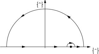
The factor exp{−ω2(t − t )} is bounded in the upper half of the complex plane for t − t > 0 and in the lower half plane for t − t < 0, and Gˆ (t − t ) is finite for all t − t . The required causality (Eq. (3.2.3)) hence limits Gˆ (ω)ˆ to the upper half of the ωˆ plane. Let us consider a contour shown in Fig. 3.1 with a small indentation near to the frequency ω0. Because the function is analytic (i.e. no poles) in the upper half plane, Cauchy’s theorem applies:
" Gˆ (ωˆ ) dωˆ = 0 .
C ωˆ − ωˆ 0
For a detailed discussion of the essential requirements and properties of the response function Gˆ (ω)ˆ , for example its boundedness and linearity, see [Bod45, Lan80], for instance. While the integral over the large semicircle vanishes4 as Gˆ (ωˆ ) → 0 when ωˆ → ∞, the integral over the small semicircle of radius η can be evaluated using ωˆ = ωˆ 0 − η exp{iφ}; then, by using the general relation
4 This is not a serious restriction since we can redefine Gˆ in the appropriate way as Gˆ (ω) − Gˆ (∞).
3.2 Kramers–Kronig relations and sum rules |
59 |
Im |
ω |
|
|
|
|
0 |
ω0 |
Re |
ω |
Fig. 3.1. Integration contour in the complex frequency plane. The limiting case is considered where the radius of the large semicircle goes to infinity while the radius of the small semicircle around ω0 approaches zero. If the contribution to the integral from the former one vanishes, only the integral along the real axis from −∞ to ∞ remains.
(sometimes called the Dirac identity) |
|
|
|
|
|
|
|
|
|
|
|||
η→0 |
1 |
= P |
1 |
i |
|
x |
|
|
(3.2.7) |
||||
x ± iη |
x |
|
|
|
|||||||||
lim |
|
|
|
|
|
|
|
|
π δ( |
|
) |
, |
|
we obtain |
|
|
|
|
|
|
|
|
|
|
|
|
|
η→0 "η |
G(ω ) |
= −i |
|
Gˆ ˆ 0 |
|
|
|
|
|||||
ωˆ −ˆωˆ |
0 d ˆ |
|
|
|
|
|
|||||||
lim |
ˆ |
|
ω |
|
|
|
π |
|
(ω |
) . |
|
|
|
|
|
|
|
|
|
|
|
||||||
This integral along the real frequency axis gives the principal value P. Therefore
|
1 |
|
∞ |
ˆ |
|
||
|
|
G(ω ) |
|
||||
Gˆ |
(ω) = |
|
P |
−∞ |
|
dω , |
(3.2.8) |
iπ |
ω − ω |
||||||
where we have omitted the subscript of the frequency ω0. In the usual way, the complex response function Gˆ (ω) can be written in terms of the real and imaginary parts as Gˆ (ω) = G1(ω) + iG2(ω), leading to the following dispersion relations between the real and imaginary parts of the response function:
|
|
1 |
|
|
|
∞ G (ω ) |
|
|
|
|
|||
G1(ω) |
= |
|
|
P |
−∞ |
2 |
dω |
(3.2.9a) |
|||||
|
π |
ω − ω |
|||||||||||
|
|
|
|
1 |
|
|
∞ G (ω ) |
|
|
||||
G2(ω) |
= |
− |
|
P |
−∞ |
1 |
|
dω ; |
(3.2.9b) |
||||
π |
ω − ω |
||||||||||||
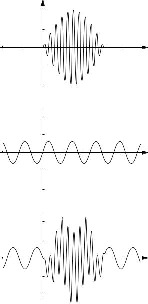
i.e. G1 and G2 are Hilbert transforms of each other. Using these general relations we can derive various expressions connecting the real and imaginary parts of different optical parameters and response functions discussed earlier. The relationship between causality and the dispersion relations is also illustrated in Fig. 3.2. Thus
60 |
3 General properties of the optical constants |
|
||||
|
Input A |
|
|
|
|
|
|
1 |
|
|
|
|
|
|
0.5 |
|
|
|
|
|
−2 |
−1 |
1 |
2 |
3 |
4 |
Time |
|
|
|
|
|
|
|
−0.5
−1
Component B 
|
1 |
|
|
|
|
|
0.5 |
|
|
|
|
−2 −1 |
1 |
2 |
3 |
4 |
Time |
|
|
|
|
|
−0.5
−1
Output A – B 
|
1 |
|
|
|
|
|
0.5 |
|
|
|
|
−2 −1 |
1 |
2 |
3 |
4 |
Time |
|
|
|
|
|
−0.5
−1
Fig. 3.2. Connection between causality and dispersion visualized by a wave package. An input A(t) which is zero for times t < 0 is formed as a superposition of many Fourier components such as B, each of which extends from t = −∞ to t = ∞. It is impossible to design a system which absorbs just the component B(t) without affecting other components; otherwise the output would contain the complement of B(t) during times before the onset of the input wave, in contradiction with causality. The lower panel shows the result of a simple subtraction of one component A(t) − B(t) which is non-zero for times t < 0 (after [Tol56]).

3.2 Kramers–Kronig relations and sum rules |
61 |
causality implies that absorption of one frequency ω must be accompanied by a compensating shift in phase of other frequencies ω ; the required phase shifts are prescribed by the dispersion relation. The opposite is also true: a change in phase at one frequency is necessarily connected to an absorption at other frequencies.
Let us apply these relations to the various material parameters and optical constants. The current J is related to the electric field E by Ohm’s law (2.2.11); and the complex conductivity σˆ (ω) = σ1(ω) + iσ2(ω) is the response function describing this. The dispersion relation which connects the real and imaginary parts of the complex conductivity is then given by
|
|
1 |
|
|
|
∞ σ2(ω ) |
|
|||||
σ1(ω) |
= |
|
|
|
P |
−∞ |
|
|
dω |
(3.2.10a) |
||
|
π |
ω − ω |
||||||||||
|
|
|
|
1 |
|
∞ σ1(ω ) |
|
|||||
σ2(ω) |
= |
− |
|
|
P −∞ |
|
dω . |
(3.2.10b) |
||||
π |
ω − ω |
|||||||||||
We can write these equations in a somewhat different form in order to eliminate the negative frequencies. Since σˆ (ω) = σˆ (−ω) from Eq. (3.2.4c), the real part σ1(−ω) = σ1(ω) is an even function and the imaginary part σ2(−ω) = −σ2(ω) is an odd function in frequency. Thus, we can rewrite Eqs (3.2.10a) and (3.2.10b) by using the transformation for a function f (x)
∞ f (x) |
dx |
|
∞ x[ f (x) |
− |
f ( |
x)] + a[ f (x) + f ( |
− |
x)] |
dx , |
|||||||||
|
|
|
|
|
|
|
|
|
||||||||||
P −∞ x − a |
= P 0 |
|
|
|
|
|
|
|
|
|
|
|||||||
|
|
|
|
|
|
|
− x2 − a2 |
|
|
|
||||||||
yielding for the two components of the conductivity |
|
|
|
|
||||||||||||||
|
|
|
|
|
2 |
|
|
0 |
∞ ω σ2(ω ) |
|
|
|
|
|||||
|
|
|
σ1(ω) |
= |
|
|
|
P |
|
|
|
dω |
|
|
(3.2.11a) |
|||
|
|
|
|
π |
ω 2 − ω2 |
|
|
|||||||||||
|
|
|
|
|
|
|
2ω |
|
|
∞ |
σ1(ω ) |
|
|
|
|
|||
|
|
|
σ2(ω) |
= |
− |
|
|
P 0 |
|
dω . |
|
|
(3.2.11b) |
|||||
|
|
|
π |
|
ω 2 − ω2 |
|
|
|||||||||||
The dispersion relations are simple integral formulas relating a dispersive process (i.e. a change in phase of the electromagnetic wave, described by σ2(ω)) to an absorption process (i.e. a loss in energy, described by σ1(ω)), and vice versa.
Next, let us turn to the complex dielectric constant. The polarization P in response to an applied electric field E leads to a displacement D given by Eq. (2.2.5), and
4π P(ω) = [ˆ(ω) − 1]E(ω) ;
consequently ˆ(ω) − 1 is the appropriate response function:
1(ω) − 1 = |
2 |
P |
0 |
∞ ω 2(ω ) |
dω |
(3.2.12a) |
|
π |
|
ω 2 − ω2 |
|||||

62 3 General properties of the optical constants
|
(ω) |
= − |
2 |
|
0 |
∞ |
ω 2[ 1(ω ) − 1] |
dω . |
(3.2.12b) |
π ω P |
|
||||||||
2 |
|
|
ω 2 − ω2 |
|
|||||
One immediate result of the dispersion relation is that if we have no absorption in the entire frequency range ( 2(ω) = 0), then there is no frequency dependence of the dielectric constant: 1(ω) = 1 everywhere. Using
|
|
|
|
|
|
|
P 0 |
∞ |
|
|
|
|
|
1 |
|
|
|
dω = 0 |
, |
|
|
|
|
|
(3.2.13) |
||||||
|
|
|
|
|
|
|
|
|
|
|
|
|
|
|
|
|
|
|
|||||||||||||
|
|
|
|
|
|
|
|
|
ω 2 − ω2 |
|
|
||||||||||||||||||||
Eq. (3.2.12b) can be simplified to |
|
|
|
|
|
|
|
|
|
|
|
|
|
|
|
|
|
|
|
|
|
||||||||||
∞ |
ω 2[1 − 1(ω )] |
dω |
= |
∞ |
[1 − 1(ω )]ω 2 − ω2 + 1(ω )ω2 − 1(ω )ω2 |
dω |
|||||||||||||||||||||||||
0 |
|
ω 2 − ω2 |
|
|
0 |
|
|
|
|
|
|
|
|
|
|
|
|
|
|
ω 2 − ω2 |
|
|
|
|
|||||||
|
|
|
|
|
|
|
|
∞ [1 |
− |
1(ω )](ω 2 − ω2) − 1(ω )ω2 |
dω |
||||||||||||||||||||
|
|
|
|
|
|
|
= 0 |
|
|
|
|
|
|
|
|
|
|
|
ω 2 − ω2 |
|
|
|
|
||||||||
|
|
|
|
|
|
|
|
|
|
|
|
|
|
|
|
|
|
|
|
|
|
|
|
||||||||
|
|
|
|
|
|
|
|
∞ |
|
|
|
|
|
|
|
|
|
|
|
|
|
∞ 1(ω )ω2 |
|
|
|
|
|||||
|
|
|
|
|
|
|
= 0 |
[1 − 1(ω )] dω − 0 |
|
|
|
dω . |
|||||||||||||||||||
|
|
|
|
|
|
|
|
ω 2 − ω2 |
|||||||||||||||||||||||
The dc |
conductivity calculated from Eq. (3.2.11a) by setting ω |
= |
0 and using |
||||||||||||||||||||||||||||
|
ω |
|
|
|
|
|
|
|
|
|
|
|
|
|
|
|
|
|
|
|
|
|
|
|
|
|
|||||
σ2 = (1 |
− 1) |
|
|
from Table 2.1 is given by |
|
|
|
|
|
|
|
|
|
|
|||||||||||||||||
4π |
[1 − 1(ω )] dω ; |
|
|
(3.2.14) |
|||||||||||||||||||||||||||
|
|
|
|
|
σdc = σ1(0) = 2π 2 |
0 |
∞ |
|
|
||||||||||||||||||||||
|
|
|
|
|
|
|
|
|
|
|
|
|
|
1 |
|
|
|
|
|
|
|
|
|
|
|
|
|
|
|
|
|
we consequently find for Eq. (3.2.12b) |
|
|
|
|
|
|
|
|
|
|
|
|
|
|
|||||||||||||||||
|
|
|
|
|
|
|
|
4π σdc |
|
|
|
2ω |
|
|
∞ |
1(ω ) |
|
|
|
|
|||||||||||
|
|
|
|
|
2(ω) = |
|
|
|
|
− |
|
|
|
P 0 |
|
dω . |
|
|
(3.2.15) |
||||||||||||
|
|
|
|
|
ω |
|
|
|
|
π |
|
ω 2 − ω2 |
|
|
|||||||||||||||||
For σdc = 0 the imaginary part of the dielectric constant diverges for ω → 0. For insulating materials σdc vanishes, and therefore the first term of the right hand side is zero. In this case by using Eq. (3.2.13) we can add a factor 1 to Eq. (3.2.15) and obtain a form symmetric to the Kramers–Kronig relation for the dielectric constant (3.2.12a):
2 |
|
= − π P 0 |
∞ |
ω 2 − ω2 |
; |
|
||
|
(ω) |
|
2ω |
1(ω ) − 1 |
dω |
|
(3.2.16) |
|
|
|
|
|
|||||
it should be noted that this expression is valid only for insulators.
For longitudinal fields the loss function 1/ ˆL(ω) describes the response to the longitudinal displacement as written in Eq. (3.1.23). Consequently 1/ ˆL(ω) can also be regarded as a response function with its components obeying the Kramers– Kronig relations
Re |
1 |
|
− 1 = |
1 |
|
−∞ |
Im |
1 |
|
|
dω |
|
(3.2.17a) |
|
|
|
|
|
|
|
|
|
|||||||
ˆ |
π P |
ˆ |
ω |
− |
||||||||||
(ω) |
∞ |
(ω ) |
|
ω |
||||||||||
|
|
3.2 |
Kramers–Kronig relations and sum rules |
|
|
|
|
63 |
||||||||||
Im |
|
1 |
|
= |
1 |
P |
∞ |
1 |
− Re |
|
1 |
|
dω |
|
|
. (3.2.17b) |
||
|
|
|
|
|
|
|
||||||||||||
(ω) |
π |
−∞ |
(ω ) |
ω |
− |
ω |
||||||||||||
|
|
|
ˆ |
|
|
|
|
|
|
|
ˆ |
|
|
|
|
|||
Similar arguments can be used for other optical constants which can be regarded as a response function. Thus the Kramers–Kronig relations for the two components of the complex refractive index Nˆ (ω) = n(ω) + ik(ω) are as follows:
|
|
2 |
|
∞ ω k(ω ) |
|
|
|
||||
n(ω) − 1 |
= |
|
|
P 0 |
|
|
|
dω |
(3.2.18a) |
||
|
π |
ω 2 − ω2 |
|||||||||
|
= |
− |
π ω P |
0 |
ω 2 − ω2 |
|
|||||
k(ω) |
|
|
|
2 |
|
|
∞ |
(ω )2 |
[n(ω ) − 1] |
dω . |
(3.2.18b) |
|
|
|
|
|
|
|
|
|
|||
This is useful for experiments which measure only one component such as the absorption α(ω) = 2k(ω)ω/c. If this is done over a wide frequency range the refractive index n(ω) can be calculated without separate phase measurements. The square of the refractive index Nˆ 2 = (n2 − k2) + 2ink is also a response function.
We can write down the dispersion relation between the amplitude √R = |rˆ| and the phase shift φr of the wave reflected off the surface of a bulk sample as in Eq. (2.4.12): Ln rˆ(ω) = ln |rˆ(ω)| + iφr(ω). The dispersion relations
|
|
1 |
|
|
|
|
∞ φ (ω ) |
|
|
|
||||
ln |rˆ(ω)| |
= |
|
|
|
P |
−∞ |
r |
dω |
(3.2.19a) |
|||||
|
π |
ω − ω |
||||||||||||
|
|
|
|
1 |
|
|
∞ ln r(ω ) |
|
|
|
||||
φr(ω) |
= |
− |
|
|
P |
−∞ |
| ˆ |
| |
dω |
(3.2.19b) |
||||
π |
ω − ω |
|
||||||||||||
follow immediately. The response function which determines the reflected power is given by the square of the reflectivity (Eq. (2.4.15)) and therefore the appropriate dispersion relations can be utilized.
Finally, the real and imaginary parts of the surface impedance Zˆ S are also related by similar dispersion relations:
|
|
|
1 |
|
|
|
|
∞ XS(ω ) |
2 |
|
|
∞ ω XS(ω ) |
|
||||||
RS(ω) − Z0 |
= |
|
P |
−∞ |
|
|
dω = |
|
|
P 0 |
|
|
dω |
||||||
π |
ω − ω |
π |
|
ω 2 − ω2 |
|||||||||||||||
S |
|
= − π P |
−∞ |
|
ω − ω |
|
|
|
|
|
|
|
|||||||
X |
(ω) |
|
|
1 |
|
|
|
∞ |
[RS(ω ) − Z0] |
dω |
|
|
(3.2.20a) |
||||||
= − π |
|
P 0 |
|
|
|
|
|||||||||||||
|
|
|
|
ω 2 − ω2 |
|
|
|
|
|
|
|
||||||||
|
|
|
|
2ω |
|
|
∞ |
[RS(ω ) − Z0] |
dω |
. |
(3.2.20b) |
||||||||
|
|
|
|
|
|
|
|
|
|
||||||||||
For the same reasons as discussed above, the difference from the free space impedance RS(ω) − Z0 has to be considered, since only this quantity approaches zero at infinite frequencies.
64 |
3 General properties of the optical constants |
Response function G
2
1
0
−1
2
1
0
−1
−20
G1
G2
G1
(a)
G2
G1
(b)
2 |
4 |
6 |
8 |
10 |
|
Frequency ω / ω0 |
|
|
|
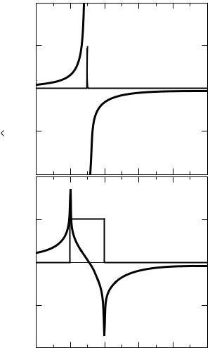
Fig. 3.3. Frequency dependence of the complex response function Gˆ (ω) = G1(ω) + iG2(ω). (a) For G2(ω) = δ{3ω0} (solid line) the corresponding component G1(ω) diverges as 1/(3ω0 − ω) (dashed line). (b) The relationship between the real and imaginary parts of a response function if G2(ω) = 1 for 2 < ω < 4 and zero elsewhere.
The Kramers–Kronig relations are non-local in frequency: the real (imaginary) component of the response at a certain frequency ω is related to the behavior of the imaginary (real) part over the entire frequency range, although the influence of the contributions diminishes as (ω 2−ω2)−1 for larger and larger frequency differences. This global behavior leads to certain difficulties when these relations are used to

3.2 Kramers–Kronig relations and sum rules |
65 |
analyze experimental results which cover only a finite range of frequencies. Certain qualitative statements can, however, be made, in particular when one or the other component of the response function displays a strong frequency dependence near certain frequencies.
From a δ-peak in the imaginary part of Gˆ (ω) we obtain a divergency in G1(ω), and vice versa, as displayed in Fig. 3.3. Also shown is the response to a pulse in G2(ω). A quantitative discussion can be found in [Tau66, Vel61].
3.2.2 Sum rules
We can combine the Kramers–Kronig relations with physical arguments about the behavior of the real and imaginary parts of the response function to establish a set of so-called sum rules for various optical parameters.
The simplest approach is the following. For frequencies ω higher than those of the highest absorption, which is described by the imaginary part of the dielectric constant 2(ω ), the dispersion relation (3.2.12a) can be simplified to
1(ω) ≈ 1 − |
2 |
0 |
∞ ω 2(ω ) dω . |
(3.2.21) |
π ω2 |
In order to evaluate the integral, let us consider a model for calculating the dielectric constant; in Sections 5.1 and 6.1 we will discuss such models for absorption processes in more detail. For a particular mode in a solid, at which the rearrangement of the electronic charge occurs, the equation of motion can, in general, be written as
m |
d2r |
+ |
|
1 dr |
+ ω02r = −eE(t) , |
(3.2.22) |
||
|
|
|
|
|
||||
dt2 |
τ dt |
|||||||
where 1/τ is a phenomenological damping constant, ω0 is the characteristic frequency of the mode, and −e and m are the electronic charge and mass, respectively. In response to the alternating field E(t) = E0 exp{−iωt}, the displacement is then given by
r = − |
eE |
1 |
. |
(3.2.23) |
|
|
|
|
|||
m |
ω02 − ω2 − iω/τ |
||||
The dipole moment of the atom is proportional to the field and given by −er = αˆ E if we have only one atom per unit volume; α(ω)ˆ is called the molecular polarizability. In this simple case the dielectric constant can now be calculated as
ˆ(ω) = 1 + 4π αˆ = 1 + |
4π e2 |
1 |
. |
(3.2.24) |
|
m |
|
ω02 − ω2 − iω/τ |
|||
Each electron participating in the absorption process leads to such a mode; in total
66 |
3 General properties of the optical constants |
we assume N modes per unit volume in the solid. At frequencies higher than the highest mode ω ω0 > 1/τ , the excitation frequency dominates the expression for the polarizability; hence the previous equation can be simplified to
lim |
|
(ω) |
|
|
4π N e2 |
|
|
ωp2 |
|
|||
= 1 − |
|
mω2 = |
1 − ω2 |
(3.2.25) |
||||||||
ω ω0 |
1 |
|
|
|||||||||
for all modes, with the plasma frequency defined as |
|
|
|
|||||||||
|
ωp = |
4π N e2 |
|
1/2 |
|
|
|
|||||
|
|
|
. |
|
(3.2.26) |
|||||||
|
m |
|
|
|
|
|||||||
From Eq. (3.2.25) we see that for high frequencies ω ω0 and ω > ωp, the real part of the dielectric constant 1 always approaches unity from below. Comparing the real part of this expansion with the previous expression for the high frequency dielectric constant given in Eq. (3.2.21), we obtain
|
|
π |
ωp2 = |
0 |
∞ |
|
|
|
||||
|
|
|
|
ω 2(ω) dω |
, |
(3.2.27) |
||||||
2 |
||||||||||||
which in terms of the optical conductivity σ1(ω) |
= (ω/4π ) 2(ω) can also be |
|||||||||||
written as |
|
|
|
|
|
|
|
|
|
|||
ω2 |
|
0 |
∞ |
|
π N e2 |
|
||||||
|
p |
= |
σ1(ω) dω = |
|
. |
(3.2.28) |
||||||
|
8 |
|
2m |
|||||||||
Therefore the spectral weight ωp2/8 defined as the area under the conductivity
spectrum |
0∞ σ1(ω) dω is proportional to the ratio of the electronic density to the |
||||||
mass of |
the electrons. |
|
|
|
|
|
|
|
! |
|
|
|
|
|
|
It can be shown rigorously that |
|
|
|
|
|||
|
|
0 |
∞ |
π |
j |
(q )2 |
(3.2.29) |
|
|
2 |
Mj j |
||||
|
|
|
|
|
|
|
|
holds for any kind of excitation in the solid in which charge is involved; here q j and M j are the corresponding charge and mass, respectively. For electrons, q = −e and M = m. For phonon excitations, for example, q may not equal e, and most importantly M is much larger than m due to the heavy ionic mass.
We still have to specify in more detail the parameter N in Eq. (3.2.26). For more than one electron per atom, N is the total number of electrons per unit volume, if the integration in Eq. (3.2.28) is carried out to infinite frequencies. This means that for high enough frequencies even the core electrons are excited, and have to be included in the sum rule. Studying the optical properties of solids, in general we are only interested in the optical response due to the conduction electrons in the case of a metal or due to the valence electrons in the case of a semiconductor. The core electron excitation energies are usually well separated in
3.2 Kramers–Kronig relations and sum rules |
67 |
the higher frequency range ω > ωc. If more than one mode is related to a single electron the polarizability sums up all contributions:
|
e2 |
f j |
|
|
|
ˆ = m j |
ω02 j − ω2 − iω/τ j |
|
(3.2.30) |
||
α(ω) |
|
|
|
. |
|
Here f j is called the oscillator strength; it measures the probability of a particular transition taking place with a characteristic frequency ω0 j . It obeys the so-called f sum rule #j f j = 1 which expresses normalization. A quantum mechanical derivation of the sum rule and a detailed discussion of the electronic transitions are given in Section 6.1.1.
Looking at the limit ω = 0, the first Kramers–Kronig relation for the dielectric
constant (3.2.12a) reads |
(0) − 1 = π 0 |
|
2ω |
|
|
|||
1 |
∞ |
dω . |
(3.2.31) |
|||||
|
|
2 |
|
|
(ω) |
|
|
|
|
|
|
|
|
|
|
|
|
The static dielectric constant is related to the sum of all higher frequency contributions of the imaginary part; it is a measure of absorption processes and their mode strength. This relation (3.2.31) is the equivalent to Eq. (3.2.14) for the dc conductivity.
Now let us consider the second Kramers–Kronig relation (3.2.12b). We can split the integral of Eq. (3.2.14), and in the case of an insulator (σdc = 0) we obtain
0 = 0 |
ωc |
∞ |
|
∞[ 1(ω) − 1] dω = 0 |
[ 1(ω) − 1] dω + ωc |
[ 1(ω) − 1] dω . (3.2.32) |
If we assume that above a cutoff frequency ωc there are no excitations (i.e. the imaginary part of the dielectric constant equals zero at frequencies higher than ωc), Eq. (3.2.25) can be applied to the second term on the right hand side of Eq. (3.2.32), yielding
∞ |
|
ωp2 |
|
ωc |
[ 1(ω) − 1] dω = |
|
. |
ωc |
|||
The rest of Eq. (3.2.32) gives
1 |
ωc |
|
|
|
2 |
|
|
|
0 |
(ω) dω |
= |
1 |
|
ωp |
|
(3.2.33) |
|
ωc |
− ωc2 |
|
||||||
|
1 |
|
|
|
, |
|||
which expresses that the average of the real part of the dielectric constant approaches unity in the high frequency limit ωc ωp.
Next, we consider a response of the electron gas to an additional electron moving inside the solid; a situation which occurs when a so-called electron loss spectroscopy experiment is conducted. The moving charge produces a displacement