Добавил:

fench Опубликованный материал нарушает ваши авторские права? Сообщите нам.

Вуз:

Национальный исследовательский ядерный университет (МИФИ)

Предмет:

Физика конденсированного тела

Файл:

Baranov.Introduction to Physics Of Ultra Cold Gases.pdf

Скачиваний:

Добавлен:

27.08.2013

Размер:

586.56 Кб

Скачать

☆

<<< < Предыдущая 1 2 3 4 5 6 7 89 / 199 10 11 12 13 14 15 16 17 18 19 > Следующая >>>

36							CHAPTER 2. BOSONS
If we compare our superﬂuid rotation with solid body rotation we get with									k = 1
I	~		I	ÑFd~l =	2p~		2p~
	~vSd~l =					Nv =		nvSc	(2.158)
		m			m		m

~	=	2	s Ñ ~vs.b.	= 2WSc:	(2.159)
~vs.b.dl		d

Here Nv and nv are the number and density of vortices respectively and Sc the area enclosed in the calculation. Substituting both equation we get

mW nv = ~p :

The velocity around one vortex is

~~ez ~r

~vs = m r2

and the total velocity is the superposition of each velocity

~s(~) = åi	m ~r		~ri	2	:
v r	~	~ez ~r ~ri
		j		j

(2.160)

(2.161)

(2.162)

2.5BEC in an isotr. harmonic trap at T=0

2.5.1 Comparison of terms in GP

+U (~r) yˆ

Hˆ = Z

d3r yˆ †

Ñ2

g Z

d3r yˆ † yˆ † yyˆ ˆ

(2.163)

mw2

4p~2

U (~r) =

g =

(2.164)

A macroscopic number of particles is in the ground state of the trap and the condensate wave function can be written as

F(~r;t) = lim			N	1 y N	i	= j(~r;t)e i	mt	(2.165)
							~
N	!	∞	h	j j

Here the braces around the limit denote that we always take the leading terms in N only. The exponential wave function carries only the trivial time dependences which arises from the different number of particles. We now get the time dependent GP (cf. (2.128)) with potential.

i~¶t j =		2	m +U (r) j + gjjj2j	(2.166)
		2~m Ñ2
	¶

2.5. BEC IN AN ISOTR. HARMONIC TRAP AT T=0

The ground state must be a stationary state. We can choose j real because if j contained a non trivial space dependent phase f(r) this would cause a gas ﬂow and therefore an increase of energy (cf. (2.142)) Thus, the equation of the ground state wave function j(~r) reads

~2 Ñ2j +U (~r)j + gj3 = mj

2m	Z d3r j2(~r) = N
n(~r) = j2

Solving this equation we get m.

The simplest case is the non-interacting gas, i.e. g = 0:

m = e0 = 2 ~w

ql03p 2

rmw

j = pNj0(~r) = pN

2l0

l0 =

(2.167)

(2.168)

(2.169)

(2.170)

If we are looking at weak interaction, we can assume the wave function to still have a similar form. Before proceeding, we have to deﬁne the term "weak". For this purpose the ratio between kinetic and potential to interaction energy has to be considered. More precisely

Ekin Epot ~wN

(2.171)

Eint

g Z

d3r j

4 =

g Z

d3r n2(r) gnN¯ = g

(2.172)

l03

~2 a N2

~wN

thus

(2.173)

int

(2.174)

kin

This ratio describes how important interaction is for the ground state wave function.

In the experiment we have l0 1mm and

23Na: a=2.75 nm 87Rb: a=5.77 nm 6Li: a=-1.45 nm (2.175)

This yields	a	10 3. Therefore we can consider the interaction to be small if
	l0

N < 1000 otherwise we have to consider the interaction right from the beginning. On the other hand we still have a gas as our criteria shows:

na¯ 3 1 )	l03 a3	=	N l0		l0		2	(2.176)
							1
	N			a		a

Our system is gaseous while N < 10003 = 109.

38	CHAPTER 2. BOSONS

2.5.2 Thomas-Fermi-Regime

Repulsive Interaction

This regime is speciﬁed by

N	a	1	(2.177)

	l0

Since we are dealing with a trapped gaseous system we assume the system to occupy a volume R3 with

R l0

(2.178)

As described in (2.174) we have

Ekin Eint gnN¯ = g

N = g

m =

¶E

¶Eint

¶N

Because of E Eint

(deﬁnition of T HOMAS-FERMI regime) and m =

mw2R2

m = g

~2a

= Nal0

mw2

= l05

) R l0

N l0

Therefore we justify (2.178)6.

(2.179)

(2.180)

¶E we get

¶N

(2.181)

(2.182)

(2.183)

(2.184)

m = g

N ~2a N

~wN

l03

= ~w N l0 ~w

Ekin

N =

N N

= ~wN N

2mR2

2ml02

6Note however, that 2 . N

. 3 in real experiments.

(2.185)

(2.186)

(2.187)

2.5. BEC IN AN ISOTR. HARMONIC TRAP AT T=0					39
Comparing this to Eint = mN we get
Ekin		N	a	34
				1	(2.188)
	mN		l0

which is consistent with (2.179). This means the kinetic energy per particle is

~w.

For numerical calculations it is convenient to use the dimensionless GP. To achieve this we set

r = l0r˜

m = ~wm

j = s

l03

(2.189)

If we insert this into the GP (2.167) we get

mw2

4p~2a

˜ 3

˜ ˜

2m l02

Ñr˜ +

l0 r˜

j +

l03 j

= ~wmj

(2.190)

~w	2		~w	2	˜	Na	˜ 3	˜ ˜
2 Ñr˜			2 r˜		˜		˜ 3	˜ ˜
2 Ñr˜		+	2 r˜		j + 4p~w l0 j			= ~wmj	(2.191)

1	2		1	2	˜	Na	˜ 3	˜ ˜
	2			2
	Ñr˜		2 r˜
2	Ñr˜	+	2 r˜		j + 4p	l0 j		= mj	(2.192)

If we are looking for the stationary ground state solution we can neglect all derivatives in (2.167) because the ground state is time independent and the kinetic terms are negligible and get

mw2r2
	j + gj3 = mj						(2.193)
2	j + gj3 = mj			, r R = w r			(2.193)
2	j2(r) = g m
			2				(2.194)
			2			m	(2.194)
		1	mw2r2		1 2m

and 0 otherwise.

Only at R numerical calculations show slight difference to our approximation. Using this, we get

N = Z

2r2

d3r j2(r) =

d3r

(2.195)

d3r

(2.196)

= g R3

4p Z0

(2.197)

dxx2(1 x2) = 4p g R3

40	CHAPTER 2. BOSONS

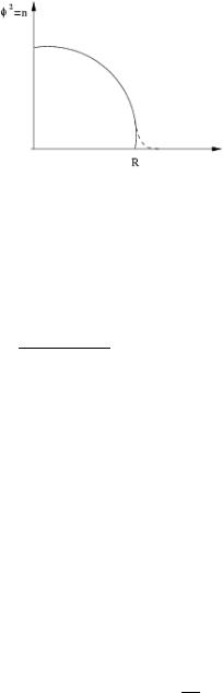
Figure 2.7: j2 = n in THOMAS-FERMI regime. The dashed line indicates the numerical solution for the radial wave function.

= 4p			4p~2a w3					m		3	15					(2.198)
= 4p			4p~2a w3					m			15					(2.198)
			mm			1			2m	2	2
			5			1
= (2m)2				p												(2.199)
= (2m)2				p	maw3~215											(2.199)
			~w			5							~w	5
=	15		~w			5		apmw =			15		~w	5	a	(2.200)
	1 2m					2		p~				1 2m		2 l0

	1						a	2
								2
								5
m =		~w 15N														(2.201)
m =	2	~w 15N					l0									(2.201)

Attractive Interaction

If we now consider the regime a < 0 we expect a collapse of the free system. If the system is in a trap, the energy levels are discrete and an equilibrium (more precisely, a long living metastable state) is possible. More quantitative (2.171) and (2.173)

Ekin		= ~wN					(2.202)
E	int		gnN¯ =	~w	N2	jaj	(2.203)
						l0

IF N is small the kinetic term can still be dominant thus preventing the collapse, i.e.

N	a	< 1	(2.204)

is necessary.

2.5. BEC IN AN ISOTR. HARMONIC TRAP AT T=0

To get a more quantitative picture we introduce a parameter z to describe possible solutions and start out with the ground state wave function of the harmonic oscillator

j(r) = p		e	r2
			2l0 z	2
	N
1			2

ql03z3pp3

The energy is now a function of z:

E(z) = E0(z) + Eint(z)

E0(z) = Z d3r j

Ñ2 +

mw r

w N

r02

2 o

p 2

r02

= ~

w N

d3r0 e

z 2Ñ2 + z2r0

e 2

p 2

d3r0 e

z 2

Ñ2

}

r022

r0 oe

+ z + z

N z

+ z

d r0 e r0

p 2

∞

r02

p 2

N z + z

dr0 r0 e

}

= ~wN

(z2 + z 2)

3{z8 p

Analogously we calculate

d3r j4 = = p2p ~wN N l0

Eint =

2 g Z

Therefore,

+ z 2) p2p

N l0

z3 o

E(z) = ~wNn4 (z2

{zx

}

(2.205)

(2.206)

(2.207)

(2.208)

(2.209)

(2.210)

(2.211)

(2.212)

(2.213)

(2.214)

Minima of this function can be obtained from this equations

~w0 N	=!	2	(z z 3) + 3x z4	=	2z4	nz5 z + 2xo =!	0	(2.215)
E (z)		3	1		3
, 0	= z(z4 1) + 2x							(2.216)

42									CHAPTER 2. BOSONS
In the limit x 1 we get
z1 2x + O(z4)									(2.217)
			1			x
z2 = 1									(2.218)
z2 = 1				2					(2.218)
The minimum value z of the expression z(z4 1) obeys the equation
(z5 z)0			= 5z4 1						(2.219)
Thus the minimum occurs at
	z	=			1				(2.220)
	z	=			1				(2.220)
					5 4
and equals
					1) =		4		(2.221)

							5	4
m := z	(z4							5

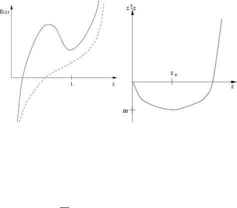
Figure 2.8: E(z) for different values of x; "- -" 2x < m and "–" 2 x > m

Therefore a solutions of (2.215) or (2.216) exists only if
					2x > m =		4	(2.222)
					2x > m =		1	(2.222)
						5 4
As a result the critical value of N is:
Nc	jaj	= p		2	= 0:671		in approximation	(2.223)
	jaj		2p	2
	l0		2p	5
	l0	5 4
					= 0:575		numerically in GP	(2.224)

2.5. BEC IN AN ISOTR. HARMONIC TRAP AT T=0

Hydrodynamic approach

From superﬂuid 4He we expect that hydrodynamics may be applicable for our system as well. The important variables in hydrodynamics are density and velocity (which is m~ ÑF in our case cf. (2.143)). We are still considering the THOMAS- FERMI-Regime (2.177). Starting out with the ansatz

y = pn(~r;t)eiΦ(~r;t)

ÑF

~vS =

(2.225)

we evaluate the the various derivatives:

¶t F

(2.226)

i~¶t y = i~eiΦ

¶t pn + ipn

= i~eiΦ

2n ¶t n + ipn ¶t F

(2.227)

= y i~

1 ¶

2n ¶t

+ i ¶t

and

(2.228)

¶n

¶F

n(Ñ2p

Ñ2y =

)eiΦ + 2(Ñp

)(ÑeiΦ)

+2p

(Ñ2eiΦ)o

(2.229)

eiΦ +

( n)i( )eiΦ

(

)

iΦ

Ñ ÑF

(i(ÑF)e

)

(2.230)

+ pn(

ÑiΦ

p y

pn (Ñ

) +

(Ñ

)(ÑF)

}

+ iÑ2F

(ÑF)2

(2.231)

to stitch the GP (2.166) together:

1 ¶n

¶F

+ i

(Ñ2pn)

(ÑF)2 +

(Ñn)(ÑF) + iÑ2F

¶t

m +U (r) + gn

(2.232)

For the imaginary part we get

1 ¶n

~2 i

(ÑnÑF + nÑ

¶t

This is the continuity equation:

¶n

+ Ñ(n~vs)

¶t

= i ~2 Ñ(nÑF):

2mn

= 0

(2.233)

(2.234)

44	CHAPTER 2. BOSONS

Evaluating the real part we get

¶F

(Ñ

) +

m +

U r

¶t

2m pn

2 s

( ) +

Differentiating this equation with respect to space coordinates (Ñ) we get

	¶~vs	+ Ñ	~2			m 2		m +U (r) + gn = 0
					Ñ2pn +
m			2mp				vs
	¶t					2
				n

(2.235)

(2.236)

	l0		Ñ
If we linearize both equations, bearing in mind N	a	1, we can neglect		pn
If we linearize both equations, bearing in mind N		1, we can neglect		pn

because we are in the THOMAS-FERMI regime were kinetic energies are small:

n = n0(~r) + dn(~r;t)					(2.237)
~		ÑF(~r;t)	2
~vs =			vs	0	(2.238)
	m

For the ground state we have (2.193)

n0(~r) =

[m U (r)]

(2.239)

which leads (2.234) and (2.236) to

dn + Ñ(n0vs) = 0 and

(2.240)

¶t

+ Ñ(U (r) m

+ gn0 +gdn) = 0

(2.241)

¶t

}

, m

vs + gÑdn = 0:

(2.242)

¶t

Differentiating again with respect to t we get

¶2

¶~v

¶2

dn + Ñ n0

dn + Ñ n0( )

Ñdn = 0

(2.243)

¶t2

¶t

¶t2

¶2

dn Ñ

n0g

Ñdn = 0

(2.244)

¶t2

|{z}

This equation can be solved for a harmonic trap ([4]). The energy remains degenerated with respect to angular momentum projection:

wnr ;l		= wp(	r + )
w	nr ;l	= w	2n2	+ 2nrl + 3nr + l		(2.245)
	nr ;l		r
	0	2n		l	non interacting case	(2.246)
		2n		l	non interacting case	(2.246)

2.5. BEC IN AN ISOTR. HARMONIC TRAP AT T=0

The solutions are quite different for the interacting and the non interacting case, e.g. for nr = 0 they are

w0;l = w l vs. w00;l = wl: (2.247)

This different behavior can be distinguished in experiments.

High energy solutions

In this case we have to formulate a more general wave function:

y(~r;t) = j(~r) + y0(~r;t)

(2.248)

Here j(r) is the ground state wave function which can be considered as a real function and y0 j describes excitations. Inserting this ansatz into the GP (2.166) and linearizing with respect to y0 we get

i~¶t y0	2
i~¶t y0	= 2~m Ñ2 m +U (r) j(r) + f:::gy0(~r;t)
¶
	+ gj2j + gj2(2y0 + y0 )
	2
	=	~	Ñ2 m +U y0 + gj2 2y0 + y0
	=	2m	Ñ2 m +U y0 + gj2 2y0 + y0

This can be solved with

y0 = u(r)e iwt + v (r)eiwt

(2.249)

(2.250)

(2.251)

(2.252)

Inserting this solution into (2.251) we get the following system of equations for u and v:

~wu =	2				u + gj2v
	~	Ñ2		m +U + 2gj2		(2.253)
	2m
~wv =	2				v + gj2u
	~		Ñ2	m +U + 2gj2		(2.254)
	2m

These are the BOGOLYUBOV-DE GENNES equations. The ui and vi are the wave function of the excitations while ~wi is the excitation energy.

A different approach for the same problem is to use the BOGOLYUBOV transformation. Since it is more extensive than in (2.3) the solution is only sketched here. We start out again with

yˆ 0(~r) = ånui(~r)a˜ i + vi (~r)a˜ i† o

(2.255)

46			CHAPTER 2. BOSONS
and require the new operators to obey	i
h	i
˜	˜ †	= di j	(2.256)
ai	;aj	= di j	(2.256)
ha˜ i;a˜ ji = ha˜ i†	;a˜ †j i	= 0	(2.257)

since we want a canonical transformation which preserves the commutator relations.

Inserting (2.255) into the commutators we get

u (~r)v (~r

0) yv0

(~r)u (0~r 0)0

= 0

(2.259)

(~r )

= 0

(2.258)

n i

(~r);y

)

åi

hyˆ 0(~r);yˆ 0† (~r 0)i = d(~r ~r 0)

(2.260)

)

åi

nui (~r)ui (~r 0) vi (~r)vi (~r 0)o = d(~r ~r 0)

(2.261)

Using the inverse transformation

ui yˆ 0(~r) viyˆ 0†

a˜ i = Z

d3r

(~r)

(2.262)

we get

d3r ui

(~r)u j (~r) vi (~r)v j (~r)

= di j

(2.263)

d3r ui(~r)v j(~r) vi(~r)u j(~r)

= 0

(2.264)

This is a mathematically rather unusual requirement, e.g. looking at (2.263) with i = j we have

d3r juij2 jvij2 = 1

The HAMILTONian can be transformed, i.e.

Hˆ = Hˆ (j) + Z

d3r yˆ 0†

Ñ2 + m +U + 2gj2

yˆ 0

g Z

d3r j2 yˆ 0

†

yˆ 0

†

+ yˆ

0yˆ

˜ †

= H(j) + const + ~åwiai

(2.265)

(2.266)

(2.267)

if and only if the ui and vi obey the BOGOLYUBOV-DE GENNES equations (2.253) and (2.254).

<<< < Предыдущая 1 2 3 4 5 6 7 89 / 199 10 11 12 13 14 15 16 17 18 19 > Следующая >>>

Соседние файлы в предмете Физика конденсированного тела

#
27.08.201310.29 Mб15Abramowitz.Stegun.Handbook of Mathematical Functions.djv
#
27.08.2013883.67 Кб8Altshuler.Simons.Universalities.From.Anderson.Localisation.to.quantum.chaos. (Les Houches Lectures).ps
#
27.08.201311.89 Mб23Ashcroft, Neil W, Mermin, David N - Solid State Physics.djvu
#
27.08.2013586.56 Кб20Baranov.Introduction to Physics Of Ultra Cold Gases.pdf
#
27.08.2013204.32 Кб14Chalker.Les.Houches. Integer quantum Hall effect & localization.pdf
#
27.08.2013463.83 Кб11Desbois.Les.Houches. Impurities and quantum Hall effect.pdf
#
27.08.2013522.31 Кб12Dotsenko.Intro to Stat Mech of Disordered Spin Systems.pdf
#
27.08.20131.68 Mб24Dresner, Stability of superconductors.2002.pdf
#
27.08.20133.91 Mб66Dressel.Gruner.Electrodynamics of Solids.2003.pdf