Добавил:

fench Опубликованный материал нарушает ваши авторские права? Сообщите нам.

Вуз:

Национальный исследовательский ядерный университет (МИФИ)

Предмет:

Физика конденсированного тела

Файл:

Baranov.Introduction to Physics Of Ultra Cold Gases.pdf

Скачиваний:

Добавлен:

27.08.2013

Размер:

586.56 Кб

Скачать

☆

<<< < Предыдущая 1 2 34 / 194 5 6 7 8 9 10 11 12 13 14 15 16 17 18 19 > Следующая >>>

1.4. BASICS OF SECOND QUANTIZATION

A general wave function can be written as a linear combination of the above functions

y	(b,f)	( ~ri ) = åpi	(b,f)	):
y		( ~ri ) = åpi	Cfpigyfpig( ri	):	(1.30)
		f g

Only the occupations ni of each single particle state are required. With this information the wave function can be reconstructed. Therefore, a simpliﬁed description can be expected if the change from ri representation to ni representation is made.

1.4Basics of second quantization

We have states n1, n2, ::: with n1, n2, ::: particles. Each state is described by jn1;n2;:::i with the special state vacuum j0;0;:::i j0i. The following operators are relevant to these states:

an is the annihilation operator: nn ! nn 1 (Note that an j0i = 0 for any n)

a†n is the creation operator: nn ! nn + 1

Note that these operators annihilate or create particles in a given quantum state unlike the operators in ﬁrst quantization which change the quantum number of one quantum state.

As was already mentioned above, there are two types of particles.

1.4.1Bosons

In this case we have the following commutation relations:

an ;an†

0 = dnn0

(1.31)

an ;an0

= an† ;an†

0 = 0

(1.32)

Because states with different n are independent, we consider only one state to understand the consequences of the above generator algebras.

The actions of the operators on the states are as follows:

aj0i = 0	a† n j0in=1anjni	(1.33)
h0jan = hnjan	a† j0i = an 1jn 1i	(1.34)

12 CHAPTER 1. GENERAL ASPECTS

All states are orthonormal, i.e. hnjmi = dnm. The an can be chosen real, as a phase can be absorbed into the deﬁnition of the states. It follows

a12 = 1

and

j0i = h0ja

n 11 + a†

a a†

j0i

(1.35)

an = h0ja

a†

(1.36)

= an2 1 + h0jan 1a† a a† j0i

j i

(1.37)

an 1 + h j

(1.38)

0 an

1a† 1 + a† a

a†

h j

n 1

† n

j i

= 2an2

1 +

0 an 1

a†

(1.39)

an 1 + h

a=j

(1.40)

0 a

= n!:

|{z}

(1.41)

Therefore each state can be written as

a†

jni

j0i

and

(1.42)

p(n

a† jni

a†

(a† )nj0i =

+ 1)!jn + 1i

(1.43)

(1.44)

= n + 1jn + 1i:

Analogously we calculate

j0i = pn! (1 + a†

a) a†

j0i

ajni = pn! a a†

(1.45)

j0i

= pn!

(n 1)!jn 1i+ a† a

a†

(1.46)

(n 1)!jn 1i+ a† (1 + a†

a) a†

j0i

(1.47)

a†

= pn!

(n 1)!jn 1i+

j0i

(1.48)

jn 1i = p

jn 1i:

(1.49)

(n 1)!

Deﬁning the particle number operator ˆn = a† a we get

n n

†

† p

n n

(1.50)

ˆ j i = a

aj i = a

j i =

and the energy operator is therefore en = ea† a.

1.4. BASICS OF SECOND QUANTIZATION

1.4.2Fermions

The operators an and a†n obey anticommutation relations

fan ;an†	0g = dnn0			(1.51)
fan ;an	0g = fan† ;an†	0g = 0	PAULI Principle:	(1.52)

Again, considering for simplicity the one state problem, it is easy to see that the occupation number N can only be 0 (the vacuum state) or 1 (PAULI principle):

aj0i = 0			aj1i = j0i a† j0i = j1i with		(1.53)
ˆ	†	a	†	a	(1.54)
H = ea			nˆ = a

1.4.3Single particle operator

We can now deﬁne the ﬁeld operators as
ˆ	åan jn (~r)	(1.55)
y(~r) =	åan jn (~r)	(1.55)
	n
yˆ † (~r) = åan† jn (~r):		(1.56)
	n

Here n runs over all states and the for a particle to be in the state n. relations:

jn (~r) are the amplitudes (probabilities) at ~r They have the following (anti-)commutation

h		i		nn0		h	0i
yˆ (~r);yˆ † (~r 0)			=	åjn (~r)jn0(~r 0)			an ;an†
			=	å	j	(~r)j (~r 0) = d(~r ~r 0)
				å	n	n
yˆ	(~r);yˆ (~r 0)			n
yˆ	(~r);yˆ (~r 0)		= hyˆ † (~r);yˆ † (~r 0)i = 0

(1.57)

(1.58)

(1.59)

By using the ﬁeld operators yˆ (~r) and yˆ † (~r) various quantum mechanical operators can easily be transformed from the space representation (~r-representation) into the occupation number representation (n-representation).

For a Single particle operator

		ˆ	N
		ˆ	= å f (~ri)	(1.60)
		F1	= å f (~ri)	(1.60)
			i=1
(Examples:
n(~r) = åd(~r ~ri) density				(1.61)
i		4i +U (~ri) Single particle HAMILTONian)
	2
Hˆ 1 = åi	~			(1.62)
Hˆ 1 = åi	2m			(1.62)

14		CHAPTER 1.			GENERAL ASPECTS
we have		nn0h		j	j	i
Z		nn0h		j	j	i		0
Fˆ1 =	d3r yˆ † (~r) f (~r)yˆ (~r) = å n		0		f	n	an†		an	(1.63)
hn0jf jni = Z	d3r0 jn†	0(~r 0) f (~r)jn (~r 0):								(1.64)

Each term in the sum on the r.h.s. of eq. (1.63) describes the transition of a particle from a state n to a state n0 with amplitude hn0jf jni.

Examples:

	ˆ †	ˆ
nˆ (~r) = y		(~r)y(~r)
ˆ		†
N	= åan an
	n
Hˆ 1	= d3r åan† 0jn0(~r)!
	Z	n0

~2	4		n
2m	4		n
		+U (~r)	åan jn (~r)

Z	n0	0	! n
=	d3r åan†		jn0(~r)	åan en jn (~r)
n			Z	d3r jn0(~r)jn (~r) = dnn	0
= åen an† an			with	d3r jn0(~r)jn (~r) = dnn

(1.65)

(1.66)

(1.67)

(1.68)

(1.69)

1.4.4 Two particle operator

	ˆ					(1.70)
	Fi = å f (~r j;~rk)					(1.70)
		j6=k
Example:
	ˆ	1
	Hint =	2 åUI		(~ri	~r j)	(1.71)
			i6= j
Now we have
Fˆ2 = Z	d3rd3r0 yˆ † (~r)yˆ † (~r 0) f (~;~r r 0)yˆ (~r 0)yˆ (~r)					(1.72)

and the the interaction part of the HAMILTONian as example:

Hˆ

0 n

0 U n

a†

with

(1.73)

int

2j Ij 1

n10

n20

;n2;n10 ;n20

0 n0 U

d3rd3r0 j

(~r)j

(~r

0)U (~r

~r 0)j

(~r 0)j

(~r)

(1.74)

1 2j Ij

n10

n20

1.4. BASICS OF SECOND QUANTIZATION

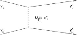
Figure 1.1: Interchange of quantum state

This term describes the scattering of two particles in initial states n1 and n2 into ﬁnal states n10 and n20 with an amplitude hn10 n20 jUIjn2n1i.

We can now write down the complete HAMILTONoperator in the form:

Hˆ

a†

0 n0 U n

a†

with

(1.75)

1 2j Ij 2

n10

n20

n1;n2;n10 ;n20

†

(1.76)

N =

åan an

The constraint of ﬁxed N introduces technical difﬁculties. introduce the chemical potential m

ˆ ! ˆ ˆ

H H mN

To avoid them, we

(1.77)

and keep a ﬁxed ¯n. The system can be thought as connected with a reservoir and the chemical potential governs the exchange process. In our calculations we have to replace

en ! en m

to take this extra term into account.

If we consider the homogeneous case then n becomes ~p and

	i ~p ~r			Z	d3 p
jn = e ~		n	!
					(2p~)
		å		V	3
en =	p2	hjn jjn0i ! (2p~)3d(~p ~p0):
	2m

(1.78)

(1.79)

(1.80)

For the time being we set the volume V 1. Since we consider the homogeneous case ~p is conserved therefore

~p	0~p	0	U ~p	~p	2i	= (2p	~	)3d(~p	1	+~p	2	~p	0		~p	0)g:	(1.81)
h	1	2	j Ij 1		2i		~		1		2		1			2

16	CHAPTER 1. GENERAL ASPECTS

To calculate g we have to switch carefully to the center of mass reference system and use relative coordinates. Then g turns out to be the FOURIER transform of

UI(~r):

g = d3rUI(~r)ei(~p1 ~p2)~~r : (1.82)

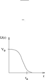
But quantum degenerate cold gases, eqn. (1.1)-(1.3), imply collisions of particles with low momenta (i.e. slow particles, r0 p ~). From scattering theory we know that in this regime collisions are characterized by only one parameter, the scattering length a. Therefore, in the BORN approximation,

g =	4p~2	(1.83)
	a:

As a result, the HAMILTONian takes the form

		e~p m a†pap +	1
Hˆ	= å~p	e~p m a†pap +	2 g p1;på2;p10 ;p20	a†p10 a†p20 ap2 ap1 :	(1.84)

Figure 1.2: Plot of inter atomic potential

<<< < Предыдущая 1 2 34 / 194 5 6 7 8 9 10 11 12 13 14 15 16 17 18 19 > Следующая >>>

Соседние файлы в предмете Физика конденсированного тела

#
27.08.201310.29 Mб15Abramowitz.Stegun.Handbook of Mathematical Functions.djv
#
27.08.2013883.67 Кб8Altshuler.Simons.Universalities.From.Anderson.Localisation.to.quantum.chaos. (Les Houches Lectures).ps
#
27.08.201311.89 Mб23Ashcroft, Neil W, Mermin, David N - Solid State Physics.djvu
#
27.08.2013586.56 Кб20Baranov.Introduction to Physics Of Ultra Cold Gases.pdf
#
27.08.2013204.32 Кб14Chalker.Les.Houches. Integer quantum Hall effect & localization.pdf
#
27.08.2013463.83 Кб11Desbois.Les.Houches. Impurities and quantum Hall effect.pdf
#
27.08.2013522.31 Кб12Dotsenko.Intro to Stat Mech of Disordered Spin Systems.pdf
#
27.08.20131.68 Mб24Dresner, Stability of superconductors.2002.pdf
#
27.08.20133.91 Mб66Dressel.Gruner.Electrodynamics of Solids.2003.pdf