Добавил:

fench Опубликованный материал нарушает ваши авторские права? Сообщите нам.

Вуз:

Национальный исследовательский ядерный университет (МИФИ)

Предмет:

Физика конденсированного тела

Файл:

Baranov.Introduction to Physics Of Ultra Cold Gases.pdf

Скачиваний:

Добавлен:

27.08.2013

Размер:

586.56 Кб

Скачать

☆

<<< < Предыдущая 1 2 3 4 5 6 7 8 910 / 1910 11 12 13 14 15 16 17 18 19 > Следующая >>>

Chapter 3

Fermions

3.1Free Fermions

3.1.1General properties

We describe our particles by their momenta ~p and some other quantum numbers a which might represent spin projections or hyper ﬁne states. The other quantum numbers have g possible values (labeled j) in total. For now, our energy depends only on ~p, i.e. we do not consider effects like spin-orbit splitting. In the free gas case we get

ep =	p2			and			(3.1)
	2m
				1
nf(~p;T ) =							(3.2)

	exp			3 T		+ 1
				ep m
n = Z			d p
					nf(~p;T )		(3.3)
		(2p~)3
Since n remains ﬁxed the last equation deﬁnes						m(T ).	At T = 0 we call m(T =

0) = eF the FERMI energy.

All states with p pF = 2meF are occupied. The reason for this is the PAULI

most 1 occupation of each single particle quantum state

principle which allows at p

(or at most g particles in an energy level which is g times degenerate):

n = g Z

Θ(eF ep) =

g Z0

d p p

= g

(3.4)

(2p~)3

6p2~3

= g

(2meF)2

eF = eF(n) only

(3.5)

6p2~3

48	CHAPTER 3. FERMIONS

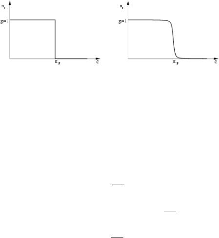
Figure 3.1: FERMI-DIRAC-Distribution at T = 0 (left) and at 0 < T eF (right)

E0 = g Z	d3 p	Θ (eF	ep)	p2		= n	3	eF	(3.6)
	(2p~)3			2m			5

If we now consider low temperatures, i.e. 0 < T eF we get the following distribution:

Here m(T;n) 6= eF. We rather get

n = g Z

d3 p

(3.7)

(2p~)3

exp

e m

+ 1

∞

= Z0

de g Z

d(e ep)

(3.8)

(2p~)3

exp

e m

+ 1

∞

= Z0

de n(e)

(3.9)

exp

e m

+ 1

where the density of states n(e) is

n(e) = g Z

d3 p

(3.10)

(2p~)3

∞

= g

d p p2d e

(3.11)

(2p~)3

2~3 mp2m

(3.12)

∞

= g

mp(e)

(3.13)

2me

2p2~3

Looking again at ﬁgure (3.1) we see, that only the region around eF is of interest. Since n(e) is analytic and smooth for e close to eF we can generally consider for

3.1. FREE FERMIONS

every analytic function f (e):

∞

= Z

∞

de f (e)

m dx

f (m + x)

(3.14)

exp

e m

+ 1

exp

+ 1

∞

= Z0

dx f (m + x)

exp

+ 1

+ Z0

dx f (m x)

(3.15)

exp

+ 1

∞

= Z0

dx f (m + x)

+ Z0

exp

+ 1

dx f (m x)

exp

+ 1

de f (e)

dx f (m x)

|{z}

(3.16)

(3.17)

+ Z0

∞

[ f (m + x) f (m x)]

exp

+ 1

∞

de f (e) + 2 f 0(m)Z0

(3.18)

exp

+ 1

Here we deﬁned

Z ∞

dx x

∞

= Z0

de f (e) + 2T 2 f 0(m)Z0

ex + 1

= Z0m de f (e) +

T 2 f 0(m)

x = e m and used

for (3.15)

e x + 1

ex + 1

m T ) m ∞ last term in (3.16)

∞

( 1)n+1e nx

∞

( 1)n+1

n=1

∞

= å

(2k)2

n=1

k=1

∞

in (3.19)

n=1

(3.19)

(3.20)

(3.21)

(3.22)

(3.23)

(3.24)

(3.25)

50	CHAPTER 3. FERMIONS

Using this so called SOMMERFELD expansion we can now calculate the particle density n:

m(T )

eF+d m

n = Z

de n(e) +

T 2

e=n =

de n(e) +

T 2

e=n

(3.26)

e=n

de n(e)+d m n(eF) +

T 2

(3.27)

| {z }

which means

2	T 2 de		e=eF
, d m n(eF) + p6	T 2 de		e=eF
		dn


(3.13):		dn	e=eF
(3.13):		de	e=eF

= 0 and

= 2eF n(eF)

(3.28)

(3.29)

which leads to the shift in the chemical potential

d m =	p2 T 2		= eF	p2	T	2

	12	eF		12	eF

Using this, we can now calculate the energy using (3.20) with

∞

E(T ) = Z0

de n(e)e

exp

e m

+ 1

m=eF+d m

(en(e)) e=n

= Z0

de n(e)e +

T 2

= Z0

de n(e)e +d m(eFn(eF))

{z0

}

(3.30)

f (e) = en(e)

(3.31)

(3.32)

(

)

T 2

n(eF) + eF ¶e

e=eF

(3.33)

+ p6

¶n

2 ¶n

= E0 +

n(eF) + eF

e=eF #

(3.34)

"d mn(eF) +

¶e

}

=0 (3.28)

<<< < Предыдущая 1 2 3 4 5 6 7 8 910 / 1910 11 12 13 14 15 16 17 18 19 > Следующая >>>

Соседние файлы в предмете Физика конденсированного тела

#
27.08.201310.29 Mб15Abramowitz.Stegun.Handbook of Mathematical Functions.djv
#
27.08.2013883.67 Кб8Altshuler.Simons.Universalities.From.Anderson.Localisation.to.quantum.chaos. (Les Houches Lectures).ps
#
27.08.201311.89 Mб23Ashcroft, Neil W, Mermin, David N - Solid State Physics.djvu
#
27.08.2013586.56 Кб20Baranov.Introduction to Physics Of Ultra Cold Gases.pdf
#
27.08.2013204.32 Кб14Chalker.Les.Houches. Integer quantum Hall effect & localization.pdf
#
27.08.2013463.83 Кб11Desbois.Les.Houches. Impurities and quantum Hall effect.pdf
#
27.08.2013522.31 Кб12Dotsenko.Intro to Stat Mech of Disordered Spin Systems.pdf
#
27.08.20131.68 Mб24Dresner, Stability of superconductors.2002.pdf
#
27.08.20133.91 Mб66Dressel.Gruner.Electrodynamics of Solids.2003.pdf