
- •Copyright
- •Contents
- •About the Author
- •Foreword
- •Preface
- •Glossary
- •1 Introduction
- •1.1 THE SCENE
- •1.2 VIDEO COMPRESSION
- •1.4 THIS BOOK
- •1.5 REFERENCES
- •2 Video Formats and Quality
- •2.1 INTRODUCTION
- •2.2 NATURAL VIDEO SCENES
- •2.3 CAPTURE
- •2.3.1 Spatial Sampling
- •2.3.2 Temporal Sampling
- •2.3.3 Frames and Fields
- •2.4 COLOUR SPACES
- •2.4.2 YCbCr
- •2.4.3 YCbCr Sampling Formats
- •2.5 VIDEO FORMATS
- •2.6 QUALITY
- •2.6.1 Subjective Quality Measurement
- •2.6.2 Objective Quality Measurement
- •2.7 CONCLUSIONS
- •2.8 REFERENCES
- •3 Video Coding Concepts
- •3.1 INTRODUCTION
- •3.2 VIDEO CODEC
- •3.3 TEMPORAL MODEL
- •3.3.1 Prediction from the Previous Video Frame
- •3.3.2 Changes due to Motion
- •3.3.4 Motion Compensated Prediction of a Macroblock
- •3.3.5 Motion Compensation Block Size
- •3.4 IMAGE MODEL
- •3.4.1 Predictive Image Coding
- •3.4.2 Transform Coding
- •3.4.3 Quantisation
- •3.4.4 Reordering and Zero Encoding
- •3.5 ENTROPY CODER
- •3.5.1 Predictive Coding
- •3.5.3 Arithmetic Coding
- •3.7 CONCLUSIONS
- •3.8 REFERENCES
- •4 The MPEG-4 and H.264 Standards
- •4.1 INTRODUCTION
- •4.2 DEVELOPING THE STANDARDS
- •4.2.1 ISO MPEG
- •4.2.4 Development History
- •4.2.5 Deciding the Content of the Standards
- •4.3 USING THE STANDARDS
- •4.3.1 What the Standards Cover
- •4.3.2 Decoding the Standards
- •4.3.3 Conforming to the Standards
- •4.7 RELATED STANDARDS
- •4.7.1 JPEG and JPEG2000
- •4.8 CONCLUSIONS
- •4.9 REFERENCES
- •5 MPEG-4 Visual
- •5.1 INTRODUCTION
- •5.2.1 Features
- •5.2.3 Video Objects
- •5.3 CODING RECTANGULAR FRAMES
- •5.3.1 Input and output video format
- •5.5 SCALABLE VIDEO CODING
- •5.5.1 Spatial Scalability
- •5.5.2 Temporal Scalability
- •5.5.3 Fine Granular Scalability
- •5.6 TEXTURE CODING
- •5.8 CODING SYNTHETIC VISUAL SCENES
- •5.8.1 Animated 2D and 3D Mesh Coding
- •5.8.2 Face and Body Animation
- •5.9 CONCLUSIONS
- •5.10 REFERENCES
- •6.1 INTRODUCTION
- •6.1.1 Terminology
- •6.3.2 Video Format
- •6.3.3 Coded Data Format
- •6.3.4 Reference Pictures
- •6.3.5 Slices
- •6.3.6 Macroblocks
- •6.4 THE BASELINE PROFILE
- •6.4.1 Overview
- •6.4.2 Reference Picture Management
- •6.4.3 Slices
- •6.4.4 Macroblock Prediction
- •6.4.5 Inter Prediction
- •6.4.6 Intra Prediction
- •6.4.7 Deblocking Filter
- •6.4.8 Transform and Quantisation
- •6.4.11 The Complete Transform, Quantisation, Rescaling and Inverse Transform Process
- •6.4.12 Reordering
- •6.4.13 Entropy Coding
- •6.5 THE MAIN PROFILE
- •6.5.1 B slices
- •6.5.2 Weighted Prediction
- •6.5.3 Interlaced Video
- •6.6 THE EXTENDED PROFILE
- •6.6.1 SP and SI slices
- •6.6.2 Data Partitioned Slices
- •6.8 CONCLUSIONS
- •6.9 REFERENCES
- •7 Design and Performance
- •7.1 INTRODUCTION
- •7.2 FUNCTIONAL DESIGN
- •7.2.1 Segmentation
- •7.2.2 Motion Estimation
- •7.2.4 Wavelet Transform
- •7.2.6 Entropy Coding
- •7.3 INPUT AND OUTPUT
- •7.3.1 Interfacing
- •7.4 PERFORMANCE
- •7.4.1 Criteria
- •7.4.2 Subjective Performance
- •7.4.4 Computational Performance
- •7.4.5 Performance Optimisation
- •7.5 RATE CONTROL
- •7.6 TRANSPORT AND STORAGE
- •7.6.1 Transport Mechanisms
- •7.6.2 File Formats
- •7.6.3 Coding and Transport Issues
- •7.7 CONCLUSIONS
- •7.8 REFERENCES
- •8 Applications and Directions
- •8.1 INTRODUCTION
- •8.2 APPLICATIONS
- •8.3 PLATFORMS
- •8.4 CHOOSING A CODEC
- •8.5 COMMERCIAL ISSUES
- •8.5.1 Open Standards?
- •8.5.3 Capturing the Market
- •8.6 FUTURE DIRECTIONS
- •8.7 CONCLUSIONS
- •8.8 REFERENCES
- •Bibliography
- •Index

• |
DESIGN AND PERFORMANCE |
246 |
7.4 PERFORMANCE
In this section we compare the performance of selected profiles of MPEG-4 Visual and H.264. It should be emphasised that what is considered to be ‘acceptable’ performance depends very much on the target application and on the type of video material that is encoded. Further, coding performance is strongly influenced by encoder decisions that are left to the discretion of the designer (e.g. motion estimation algorithm, rate control method, etc.) and so the performance achieved by a commercial CODEC may vary considerably from the examples reported here.
7.4.1 Criteria
Video CODEC performance can be considered as a tradeoff between three variables, quality, compressed bit rate and computational cost. ‘Quality’ can mean either subjective or objective measured video quality (see Chapter 2). Compressed bit rate is the rate (in bits per second) required to transmit a coded video sequence and computational cost refers to the processing ‘power’ required to code the video sequence. If video is encoded in real time, then the computational cost must be low enough to ensure encoding of at least n frames per second (where n is the target number of frames per second); if video is encoded ‘offline’, i.e. not in real time, then the computational cost per frame determines the total coding time of a video sequence.
The rate–distortion performance of a video CODEC describes the tradeoff between two of these variables, quality and bit rate. Plotting mean PSNR against coded bit rate produces a characteristic rate–distortion curve (Figure 7.23). As the bit rate is reduced, quality (as measured by PSNR) drops at an increasing rate. Plotting rate–distortion curves for identical source material (i.e. the same resolution, frame rate and content) is a widely accepted method of comparing the performance of two video CODECs. As Figure 7.23 indicates, ‘better’ rate–distortion performance is demonstrated by moving the graph up and to the left.
Comparing and evaluating competing video CODECs is a difficult problem. Desirable properties of a video CODEC include good rate–distortion performance and low (or acceptable) computational complexity. When comparing CODECs, it is important to use common
better performance |
worse performance |
coded bitrate
Figure 7.23 Example of a rate–distortion curve

PERFORMANCE |
• |
|
247 |
|
test conditions where possible. For example, different video sequences can lead to dramatic differences in rate–distortion performance (i.e. some video sequences are ‘easier’ to code than others) and computational performance (especially if video processing is carried out in software). Certain coding artefacts (e.g. blocking, ringing) may be more visible in some decoded sequences than others. For example, blocking distortion is particularly visible in larger areas of continuously-varying tone in an image and blurring of features (for example due to a crude deblocking filter) is especially obvious in detailed areas of an image.
7.4.2 Subjective Performance
In this section we examine the subjective quality of video sequences after encoding and decoding. The ‘Office’ sequence (Figure 7.24) contains 200 frames, each captured in 4:2:0 CIF format (see Chapter 2 for details of this format). The ‘Office’ sequence was shot from a fixed camera position and the only movement is due to the two women. In contrast, the ‘Grasses’ sequence (Figure 7.25), also consisting of 200 CIF frames, was shot with a handheld camera and contains rapid, complex movement of grass stems. This type of sequence is particularly difficult to encode due to the high detail and complex movement, since it is difficult to find accurate matches during motion estimation.
Each sequence was encoded using three CODECs, an MPEG-2 Video CODEC, an MPEG-4 Simple Profile CODEC and the H.264 Reference Model CODEC (operating in Baseline Profile mode, using only one reference picture for motion compensation). In each case, the first frame was encoded as an I-picture. The remaining frames were encoded as
Figure 7.24 Office: original frame

• |
DESIGN AND PERFORMANCE |
248 |
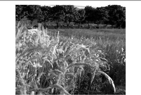
Figure 7.25 Grasses: original frame
P-pictures using the MPEG-4 and H.264 CODECs and as a mixture of B- and P-pictures with the MPEG-2 CODEC (with the sequence BBPBBP. . . ). The ‘Office’ sequence was encoded at a mean bitrate of 150 kbps with all three CODECs and the ‘Grasses’ sequence at a mean bitrate of 900 kbps.
The decoded quality varies significantly between the three CODECs. A close-up of a frame from the ‘Office’ sequence after encoding and decoding with MPEG-2 (Figure 7.26) shows considerable blocking distortion and loss of detail. The MPEG-4 Simple Profile frame (Figure 7.27) is noticeably better but there is still evidence of blocking and ringing distortion. The H.264 frame (Figure 7.28) is the best of the three and at first sight there is little difference between this and the original frame (Figure 7.24). Visually important features such as the woman’s face and smooth areas of continuous tone variation have been preserved but fine texture (such as the wood grain on the table and the texture of the wall) has been lost.
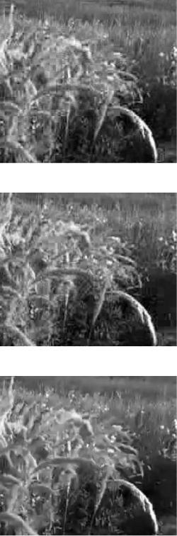
The results for the ‘Grasses’ sequence are less clear-cut. At 900 kbps, all three decoded sequences are clearly distorted. The MPEG-2 sequence (a close-up of one frame is shown in Figure 7.29) has the most obvious blocking distortion but blocking distortion is also clearly visible in the MPEG-4 Simple Profile sequence (Figure 7.30). The H.264 sequence (Figure 7.31) does not show obvious block boundaries but the image is rather blurred due to the deblocking filter. Played back at the full 25 fps frame rate, the H.264 sequence looks better than the other two but the performance improvement is not as clear as for the ‘Office’ sequence.
These examples highlight the way CODEC performance can change depending on the video sequence content. H.264 and MPEG-4 SP perform well at a relatively low bitrate (150 kbps) when encoding the ‘Office’ sequence; both perform significantly worse at a higher bitrate (900 kbps) when encoding the more complex ‘Grasses’ sequence.

Figure 7.26 Office: encoded and decoded, MPEG-2 Video (close-up)
Figure 7.27 Office: encoded and decoded, MPEG-4 Simple Profile (close-up)
Figure 7.28 Office: encoded and decoded, H.264 Baseline Profile (close-up)

Figure 7.29 Grasses: encoded and decoded, MPEG-2 Video (close-up)
Figure 7.30 Grasses: encoded and decoded, MPEG-4 Simple Profile (close-up)
Figure 7.31 Grasses: encoded and decoded, H.264 Baseline Profile (close-up)

PERFORMANCE |
• |
|
251 |
|
Office (CIF, 50 frames)
|
44 |
|
|
|
|
|
|
|
|
|
|
|
42 |
|
|
|
|
|
|
|
|
|
|
|
40 |
|
|
|
|
|
|
|
|
|
|
(dB) |
38 |
|
|
|
|
|
Office, MP4 SP |
|
|
|
|
YPSNR |
|
|
|
|
|
|
|
|
|||
|
|
|
|
|
|
Office, H.264 Baseline |
|
|
|||
36 |
|
|
|
|
|
|
|
|
|
|
|
|
|
|
|
|
|
|
|
|
|
|
|
|
34 |
|
|
|
|
|
|
|
|
|
|
|
32 |
|
|
|
|
|
|
|
|
|
|
|
30 |
|
|
|
|
|
|
|
|
|
|
|
0 |
100000 |
200000 |
300000 |
400000 |
500000 |
600000 |
700000 |
800000 |
900000 |
1000000 |
|
|
|
|
|
|
Bitrate (bps) |
|
|
|
|
|
Figure 7.32 Rate–distortion comparison: ‘Office’, CIF
7.4.3 Rate–distortion Performance
Measuring bitrate and PSNR at a range of quantiser settings provides an estimate of compression performance that is numerically more accurate (but less closely related to visual perception) than subjective comparisons. Some comparisons of MPEG4 and H.264 performance are presented here.
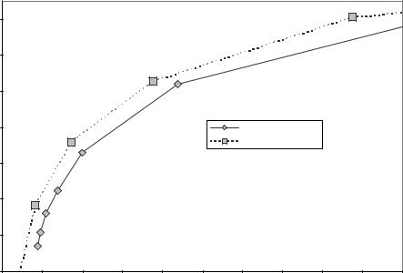
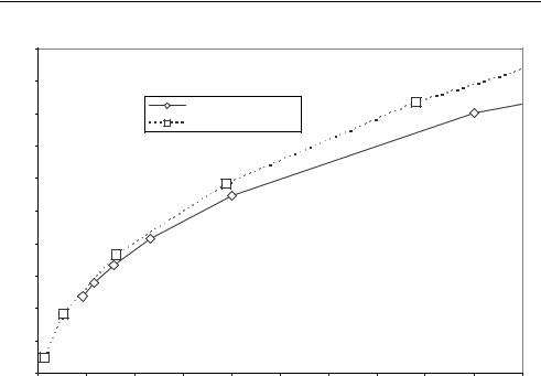
Figure 7.32 and Figure 7.33 compare the performance of MPEG4 (Simple Profile) and H.264 (Baseline Profile, 1 reference frame) for the ‘Office’ and ‘Grasses’ sequences. Note that ‘Office’ is easier to compress than ‘Grasses’ (see above) and at a given bitrate, the PSNR of ‘Office’ is significantly higher than that of ‘Grasses’. H.264 out-performs MPEG4 compression at all of the tested bit rates, but the rate-distortion gain is more noticeable for the ‘Office’ sequence.
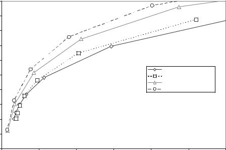
The rate–distortion performance of the popular ‘Carphone’ test sequence is plotted in Figure 7.34. This sequence contains moderate motion and in this case the source is QCIF resolution at 30 frames per second. Four sets of results are compared, two from MPEG-4 and two from H.264. The first two are MPEG-4 Simple Profile (first frame coded as an I-picture, subsequent frames coded as P-pictures) and MPEG-4 Advanced Simple Profile (using two B- pictures between successive P-pictures, no other ASP tools used). The second pair are H.264 Baseline (first frame coded as an I-slice, subsequent frames coded as P-slices, one reference frame used for inter prediction, UVLC/CAVLC entropy coding) and H.264 Main Profile (first frame coded as an I-slice, subsequent frames coded as P-slices, five reference frames used for inter prediction, CABAC entropy coding).

• |
DESIGN AND PERFORMANCE |
252 |
Grasses (CIF, 50 frames)
|
40 |
|
|
|
|
|
|
|
|
|
|
|
38 |
|
|
|
|
|
|
|
|
|
|
|
36 |
|
|
Grasses, MP4 SP |
|
|
|
|
|
||
|
|
|
Grasses, H.264 Baseline |
|
|
|
|
|
|||
|
|
|
|
|
|
|
|
|
|||
|
34 |
|
|
|
|
|
|
|
|
|
|
(dB) |
32 |
|
|
|
|
|
|
|
|
|
|
|
|
|
|
|
|
|
|
|
|
|
|
YPSNR |
30 |
|
|
|
|
|
|
|
|
|
|
28 |
|
|
|
|
|
|
|
|
|
|
|
|
|
|
|
|
|
|
|
|
|
|
|
|
26 |
|
|
|
|
|
|
|
|
|
|
|
24 |
|
|
|
|
|
|
|
|
|
|
|
22 |
|
|
|
|
|
|
|
|
|
|
|
20 |
|
|
|
|
|
|
|
|
|
|
|
0 |
500000 |
1000000 |
1500000 |
2000000 |
2500000 |
3000000 |
3500000 |
4000000 |
4500000 |
5000000 |
|
|
|
|
|
|
Bitrate (bps) |
|
|
|
|
|
Figure 7.33 Rate–distortion comparison: ‘Grasses’, CIF
MPEG-4 ASP performs slightly better than MPEG-4 SP at higher bitrates but performs worse at lower bitrates (in this case). It is interesting to note that other ASP tools (quarterpel MC and alternate quantiser) produced poorer performance in this test. H.264 Baseline outperforms both MPEG-4 profiles at all bitrates and CABAC and multiple reference frames provide a further performance gain. For example, at a PSNR of 35 dB, MPEG-4 SP produces a coded bitrate of around 125 kbps, ASP reduces the bitrate to around 120 kbps, H.264 Baseline (with one reference frame) produces a bitrate of around 80 kbps and H.264 with CABAC and five reference frames gives a bitrate of less than 70 kbps.
The results for the ‘Carphone’ sequence show a more convincing performance gain from H.264 than the results for ‘Grasses’ and ‘Office’. This is perhaps because ‘Carphone’ is a professionally-captured sequence with high image fidelity whereas the other two sequences were captured from a high-end consumer video camera and have more noise in the original images.
Other Performance Studies
The compression performance of MPEG-4 Simple and Advanced Simple Profiles are compared in [35]. In this paper the Advanced Simple tools are found to improve the compression performance significantly, producing a coded bitrate around 30–40% smaller for the same video quality, at the expense of increased encoder complexity. Most of the performance gain

PERFORMANCE |
• |
|
253 |
|
QCIF sequence ("Carphone", 200 frames)
|
45 |
|
|
|
|
|
|
|
43 |
|
|
|
|
|
|
|
41 |
|
|
|
|
|
|
|
39 |
|
|
|
|
|
|
(dB) |
37 |
|
|
|
|
|
|
|
|
|
|
|
MPEG4 SP |
|
|
PSNR |
|
|
|
|
|
|
|
35 |
|
|
|
|
MPEG4 ASP |
|
|
|
|
|
|
|
|
||
|
|
|
|
|
H264 UVLC, 1 reference |
|
|
Y |
|
|
|
|
|
|
|
33 |
|
|
|
|
H264 CABAC, 5 reference |
|
|
|
|
|
|
|
|
||
|
31 |
|
|
|
|
|
|
|
29 |
|
|
|
|
|
|
|
27 |
|
|
|
|
|
|
|
25 |
|
|
|
|
|
|
|
0 |
100000 |
200000 |
300000 |
400000 |
500000 |
600000 |
|
|
|
|
Bitrate (bps) |
|
|
|
Figure 7.34 Rate–distortion comparison: ‘Carphone’, QCIF
is due to the use of B-pictures (which require extra storage and encoding delay), quarterpixel motion compensation and rate–distortion optimised mode selection (i.e. choosing the encoding mode of each macroblock to maximise compression performance).
Reference [36] evaluates the performance of H.264 (an older version of the test model) and compares it with H.263++ (H.263 with optional modes to improve coding performance). According to the results presented, H.264 (H.26L) consistently out-performs H.263++. The authors study the contribution of some of the optional features of H.264 and conclude that CABAC provides a consistent coding gain compared with VLCs, reducing the coded bit rate by an average of 7.7% for the same objective quality (although the version of the test model did not include the more efficient context-adaptive VLCs for coefficient encoding). Using multiple reference frames for motion-compensated prediction provides better performance than a single reference frame, although the gains are slightly less obvious (a mean gain of 5.7% over the single reference frame case). Small motion compensation block sizes (down to 4 × 4) provided a clear performance gain over a single vector per macroblock (a mean bit rate saving of 16.4%), although most of the gain (13.7%) was achieved for a minimum block size of 8 × 8.
H.264 is compared with both H.263++ and MPEG-4 Visual Advanced Simple Profile in [37]. The authors compared the luminance PSNR (see Chapter 2) of each CODEC under the same test conditions. The three CODECs were chosen to represent the most highly-optimised versions of each standard available at the time. Test Model 8 of H.26L (an earlier version