


ENTROPY CODER |
• |
|
69 |
|
|
can be generated automatically (‘on the fly’) if the input symbol is known. Exponential Golomb codes (Exp-Golomb) fall into this category and are described in Chapter 6.
3.5.3 Arithmetic Coding
The variable length coding schemes described in Section 3.5.2 share the fundamental disadvantage that assigning a codeword containing an integral number of bits to each symbol is sub-optimal, since the optimal number of bits for a symbol depends on the information content and is usually a fractional number. Compression efficiency of variable length codes is particularly poor for symbols with probabilities greater than 0.5 as the best that can be achieved is to represent these symbols with a single-bit code.
Arithmetic coding provides a practical alternative to Huffman coding that can more closely approach theoretical maximum compression ratios [8]. An arithmetic encoder converts a sequence of data symbols into a single fractional number and can approach the optimal fractional number of bits required to represent each symbol.
Example
Table 3.8 lists the five motion vector values (−2, −1, 0, 1, 2) and their probabilities from Example 1 in Section 3.5.2.1. Each vector is assigned a sub-range within the range 0.0 to 1.0, depending on its probability of occurrence. In this example, (−2) has a probability of 0.1 and is given the subrange 0–0.1 (i.e. the first 10% of the total range 0 to 1.0). (−1) has a probability of 0.2 and is given the next 20% of the total range, i.e. the subrange 0.1−0.3. After assigning a sub-range to each vector, the total range 0–1.0 has been divided amongst the data symbols (the vectors) according to their probabilities (Figure 3.48).
Table 3.8 Motion vectors, sequence 1: probabilities and sub-ranges
Vector |
Probability |
log2 (1/ P) Sub-range |
|
−2 |
0.1 |
3.32 |
0–0.1 |
−1 |
0.2 |
2.32 |
0.1–0.3 |
0 |
0.4 |
1.32 |
0.3–0.7 |
1 |
0.2 |
2.32 |
0.7–0.9 |
2 |
0.1 |
3.32 |
0.9–1.0 |
|
|
|
|
Total range
0 |
0.1 |
|
0.3 |
0. 7 |
0.9 |
1 |
||||||
|
|
|
|
|
|
|
|
|
|
|
|
|
|
|
|
|
|
|
|
|
|
|
|
|
|
|
|
(-2 ) |
|
(-1) |
(0) |
(+1) |
|
|
(+2) |
|
||
Figure 3.48 Sub-range example

70 VIDEO CODING CONCEPTS
|
Encoding Procedure for Vector Sequence (0, |
|
1, 0, 2): |
|
||||
• |
Range |
Symbol |
|
− |
|
|
||
|
|
|
|
|
||||
|
|
|
|
|
||||
|
Encoding procedure |
(L → H) |
(L → H) |
Sub-range |
Notes |
|||
1. |
Set the initial range. |
0 → 1.0 |
|
0.3 → 0.7 |
|
|||
2. |
For the first data |
|
(0) |
|
||||
|
|
symbol, find the |
|
|
|
|
|
|
|
|
corresponding sub- |
|
|
|
|
|
|
|
|
range (Low to High). |
0.3 → 0.7 |
|
|
|
|
|
3. |
Set the new range (1) |
|
|
|
|
|
||
|
|
to this sub-range. |
|
(−1) |
0.1 → 0.3 |
|
||
4. |
For the next data |
|
This is the sub-range |
|||||
|
|
symbol, find the sub- |
|
|
|
|
|
within the interval 0–1 |
|
|
range L to H. |
0.34 → 0.42 |
|
|
|
|
|
5. |
Set the new range (2) |
|
|
|
|
0.34 is 10% of the range |
||
|
|
to this sub-range |
|
|
|
|
|
0.42 is 30% of the range |
|
|
within the previous |
|
|
|
|
|
|
|
|
range. |
|
|
0.3 → 0.7 |
|
||
6. |
Find the next sub- |
|
(0) |
|
||||
|
|
range. |
0.364→0.396 |
|
|
|
|
|
7. |
Set the new range (3) |
|
|
|
|
0.364 is 30% of the |
||
|
|
within the previous |
|
|
|
|
|
range; 0.396 is 70% of |
|
|
range. |
|
|
0.9 → 1.0 |
the range |
||
8. |
Find the next sub- |
|
(2) |
|
||||
|
|
range. |
0.3928→0.396 |
|
|
|
|
|
9. |
Set the new range (4) |
|
|
|
|
0.3928 is 90% of the |
||
|
|
within the previous |
|
|
|
|
|
range; 0.396 is 100% of |
|
|
range. |
|
|
|
|
|
the range |
|
|
|
|
|
|
|
|
|
Each time a symbol is encoded, the range (L to H) becomes progressively smaller. At the end of the encoding process (four steps in this example), we are left with a final range (L to H). The entire sequence of data symbols can be represented by transmitting any fractional number that lies within this final range. In the example above, we could send any number in the range 0.3928 to 0.396: for example, 0.394. Figure 3.49 shows how the initial range (0 to 1) is progressively partitioned into smaller ranges as each data symbol is processed. After encoding the first symbol (vector 0), the new range is (0.3, 0.7). The next symbol (vector –1) selects the sub-range (0.34, 0.42) which becomes the new range, and so on. The final symbol (vector +2) selects the subrange (0.3928, 0.396) and the number 0.394 (falling within this range) is transmitted. 0.394 can be represented as a fixed-point fractional number using nine bits, so our data sequence (0, −1, 0, 2) is compressed to a nine-bit quantity.
Decoding Procedure
|
|
|
|
Decoded |
Decoding procedure |
Range |
Sub-range |
symbol |
|
|
|
|
|
|
1. |
Set the initial range. |
0 → 1 |
0.3 → 0.7 |
|
2. |
Find the sub-range in which the |
|
(0) |
|
|
received number falls. This |
|
|
|
|
indicates the first data symbol. |
|
|
|

ENTROPY CODER |
|
|
|
71 |
|
||
|
(cont.) |
|
|
|
• |
|
|
|
|
|
|
|
Decoded |
|
|
|
Decoding procedure |
Range |
Sub-range |
symbol |
|
|
|
|
|
|
|
|
|
|
|
3. |
Set the new range (1) to this sub- |
0.3 → 0.7 |
|
|
|
|
|
|
|
range. |
|
0.34 → 0.42 |
(−1) |
|
|
4. |
Find the sub-range of the new |
|
|
|
|||
|
|
range in which the received |
|
|
|
|
|
|
|
number falls. This indicates the |
|
|
|
|
|
|
|
second data symbol. |
0.34 → 0.42 |
|
|
|
|
5. |
Set the new range (2) to this sub- |
|
|
|
|
||
|
|
range within the previous range. |
|
0.364 → 0.396 |
|
|
|
6. |
Find the sub-range in which the |
|
(0) |
|
|
||
|
|
received number falls and decode |
|
|
|
|
|
|
|
the third data symbol. |
0.364 → 0.396 |
|
|
|
|
7. |
Set the new range (3) to this sub- |
|
|
|
|
||
|
|
range within the previous range. |
|
0.3928→ 0.396 |
|
|
|
8. |
Find the sub-range in which the |
|
|
|
|
||
|
|
received number falls and decode |
|
|
|
|
|
|
|
the fourth data symbol. |
|
|
|
|
|
|
|
|
|
|
|
|
|
0 |
0.1 |
0.3 |
1 |
0.7 |
0.9 |
1 |
|||||||
|
|
|
|
|
|
|
|
|
|
|
|
|
|
|
|
|
|
|
|
|
|
(0) |
|
|
|
|
|
|
|
|
|
|
|
|
|
|
|
|
|
|
|
0.3 |
0.34 |
0.42 |
|
|
0.58 |
0.66 |
0.7 |
||||||
0 |
|||||||||||||
|
|
|
|
|
|
|
|
|
|
|
|
|
|
|
|
|
|
|
|
|
|
|
|
|
|
|
|
|
|
|
|
|
|
|
|
|
|
|
|
|
|
|
|
(-1) |
|
|
|
|
|
|
|
|
|
|
|
0.34 |
0.348 |
0.364 |
|
|
0.396 |
0.412 |
0.42 |
||||||
|
|
|
|
|
|
|
|
|
|
|
|
|
|
|
|
|
|
|
|
|
|
|
|
|
|
|
|
|
|
|
|
|
|
|
|
(0) |
|
|
|
|
|
|
|
|
|
|
|
|
|
|
|
|
|
|
|
0.364 |
0.3672 |
0.3736 |
|
0.3864 |
0.3928 |
0.396 |
|||||||
|
|
|
|
|
|
|
|
|
|
|
|
|
|
|
|
|
|
|
|
|
|
|
|
|
|
|
|
|
|
|
|
|
|
|
|
|
|
|
|
|
|
0.394
(2)
Figure 3.49 Arithmetic coding example

• |
VIDEO CODING CONCEPTS |
72 |
The principal advantage of arithmetic coding is that the transmitted number (0.394 in this case, which may be represented as a fixed-point number with sufficient accuracy using nine bits) is not constrained to an integral number of bits for each transmitted data symbol. To achieve optimal compression, the sequence of data symbols should be represented with:
log2(1/P0) + log2(1/P−1) + log2(1/P0) + log2(1/P2)bits = 8.28bits
In this example, arithmetic coding achieves nine bits, which is close to optimum. A scheme using an integral number of bits for each data symbol (such as Huffman coding) is unlikely to come so close to the optimum number of bits and, in general, arithmetic coding can out-perform Huffman coding.
3.5.3.1 Context-based Arithmetic Coding
Successful entropy coding depends on accurate models of symbol probability. Context-based Arithmetic Encoding (CAE) uses local spatial and/or temporal characteristics to estimate the probability of a symbol to be encoded. CAE is used in the JBIG standard for bi-level image compression [9] and has been adopted for coding binary shape ‘masks’ in MPEG-4 Visual (see Chapter 5) and entropy coding in the Main Profile of H.264 (see Chapter 6).
3.6 THE HYBRID DPCM/DCT VIDEO CODEC MODEL
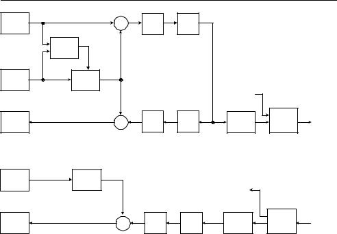
The major video coding standards released since the early 1990s have been based on the same generic design (or model) of a video CODEC that incorporates a motion estimation and compensation front end (sometimes described as DPCM), a transform stage and an entropy encoder. The model is often described as a hybrid DPCM/DCT CODEC. Any CODEC that is compatible with H.261, H.263, MPEG-1, MPEG-2, MPEG-4 Visual and H.264 has to implement a similar set of basic coding and decoding functions (although there are many differences of detail between the standards and between implementations).
Figure 3.50 and Figure 3.51 show a generic DPCM/DCT hybrid encoder and decoder. In the encoder, video frame n (Fn ) is processed to produce a coded (compressed) bitstream and in the decoder, the compressed bitstream (shown at the right of the figure) is decoded to produce a reconstructed video frame Fn . not usually identical to the source frame. The figures have been deliberately drawn to highlight the common elements within encoder and decoder. Most of the functions of the decoder are actually contained within the encoder (the reason for this will be explained below).
Encoder Data Flow
There are two main data flow paths in the encoder, left to right (encoding) and right to left (reconstruction). The encoding flow is as follows:
1.An input video frame Fn is presented for encoding and is processed in units of a macroblock (corresponding to a 16 × 16 luma region and associated chroma samples).
2. Fn is compared with a reference frame, for example the previous encoded frame (Fn−1). |
|||
A motion estimation function finds a 16 |
× |
16 region in F |
(or a sub-sample interpolated |
|
n−1 |
|
|
THE HYBRID DPCM/DCT VIDEO CODEC MODEL |
|
|
73 |
||||
Fn |
+ |
Dn |
DCT |
Quant |
|
|
• |
(current) |
- |
|
|
|
|||
|
Motion |
|
|
|
|
|
|
|
Estimate |
|
|
|
|
|
|
F’n-1 |
Motion |
P |
|
|
|
|
|
(reference) |
Compensate |
|
|
|
|
|
|
|
|
|
|
|
Vectors and |
|
|
|
|
|
|
|
headers |
|
|
|
|
+ D’ |
|
|
|
Entropy |
Coded |
F’n |
|
n |
IDCT |
Rescale |
Reorder |
||
|
|
encode |
bistream |
||||
(reconstructed) |
|
+ |
|
|
X |
|
|
|
|
|
|
|
|
||
|
Figure 3.50 DPCM/DCT video encoder |
|
|
||||
F'n-1 |
Motion |
P |
|
|
|
|
|
(reference) |
Compensate |
|
|
|
Vectors and |
|
|
|
|
|
|
|
|
||
|
|
|
|
|
|
|
|
|
|
|
|
|
headers |
|
|
F'n |
|
+ D' |
n |
|
X |
Entropy |
Coded |
|
|
|
Reorder |
||||
|
+ |
IDCT |
Rescale |
decode |
bistream |
||
(reconstructed) |
|
|
|
|
|
||
|
|
|
|
|
|
|
|
|
Figure 3.51 DPCM/DCT video decoder |
|
|
||||
version of F’n−1) that ‘matches’ the current macroblock in Fn (i.e. is similar according to some matching criteria). The offset between the current macroblock position and the chosen reference region is a motion vector MV.
3.Based on the chosen motion vector MV, a motion compensated prediction P is generated (the 16 × 16 region selected by the motion estimator).
4.P is subtracted from the current macroblock to produce a residual or difference macroblock D.
5.D is transformed using the DCT. Typically, D is split into 8 × 8 or 4 × 4 sub-blocks and each sub-block is transformed separately.
6.Each sub-block is quantised (X).
7.The DCT coefficients of each sub-block are reordered and run-level coded.
8.Finally, the coefficients, motion vector and associated header information for each macroblock are entropy encoded to produce the compressed bitstream.
The reconstruction data flow is as follows:
1.Each quantised macroblock X is rescaled and inverse transformed to produce a decoded residual D . Note that the nonreversible quantisation process means that D is not identical to D (i.e. distortion has been introduced).
2.The motion compensated prediction P is added to the residual D to produce a reconstructed
macroblock and the reconstructed macroblocks are saved to produce reconstructed frame Fn .

• |
VIDEO CODING CONCEPTS |
74 |
After encoding a complete frame, the reconstructed frame Fn may be used as a reference frame for the next encoded frame Fn+1 .
Decoder Data Flow
1.A compressed bitstream is entropy decoded to extract coefficients, motion vector and header for each macroblock.
2.Run-level coding and reordering are reversed to produce a quantised, transformed macroblock X.
3.X is rescaled and inverse transformed to produce a decoded residual D .
4.The decoded motion vector is used to locate a 16 × 16 region in the decoder’s copy of the previous (reference) frame Fn−1. This region becomes the motion compensated prediction P.
5.P is added to D to produce a reconstructed macroblock. The reconstructed macroblocks are saved to produce decoded frame Fn .
After a complete frame is decoded, Fn is ready to be displayed and may also be stored as a reference frame for the next decoded frame Fn+1.
It is clear from the figures and from the above explanation that the encoder includes a decoding path (rescale, IDCT, reconstruct). This is necessary to ensure that the encoder and decoder use identical reference frames Fn−1 for motion compensated prediction.
Example
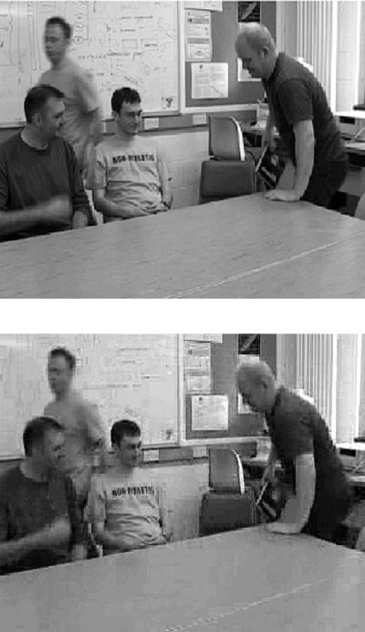
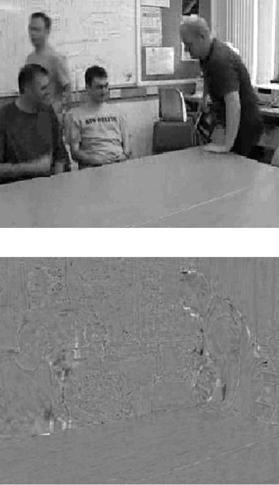
A 25-Hz video sequence in CIF format (352 × 288 luminance samples and 176 × 144 red/blue chrominance samples per frame) is encoded and decoded using a DPCM/DCT CODEC. Figure 3.52 shows a CIF (video frame (Fn ) that is to be encoded and Figure 3.53 shows the reconstructed previous frame Fn−1. Note that Fn−1 has been encoded and decoded and shows some distortion. The difference between Fn and Fn−1 without motion compensation (Figure 3.54) clearly still contains significant energy, especially around the edges of moving areas.
Motion estimation is carried out with a 16 × 16 luma block size and half-sample accuracy, producing the set of vectors shown in Figure 3.55 (superimposed on the current frame for clarity). Many of the vectors are zero (shown as dots) which means that the best match for the current macroblock is in the same position in the reference frame. Around moving areas, the vectors tend to point in the direction from which blocks have moved (e.g. the man on the left is walking to the left; the vectors therefore point to the right, i.e. where he has come from). Some of the vectors do not appear to correspond to ‘real’ movement (e.g. on the surface of the table) but indicate simply that the best match is not at the same position in the reference frame. ‘Noisy’ vectors like these often occur in homogeneous regions of the picture, where there are no clear object features in the reference frame.
The motion-compensated reference frame (Figure 3.56) is the reference frame ‘reorganized’ according to the motion vectors. For example, note that the walking person (2nd left) has been moved to the left to provide a better match for the same person in the current frame and that the hand of the left-most person has been moved down to provide an improved match. Subtracting the motion compensated reference frame from the current frame gives the motion-compensated residual in Figure 3.57 in which the energy has clearly been reduced, particularly around moving areas.
THE HYBRID DPCM/DCT VIDEO CODEC MODEL |
• |
|
75 |
|
|
Figure 3.52 Input frame Fn
Figure 3.53 Reconstructed reference frame F −
n 1
• |
VIDEO CODING CONCEPTS |
76 |
Figure 3.54 Residual Fn − Fn−1 (no motion compensation)
Figure 3.55 16 × 16 motion vectors (superimposed on frame)
THE HYBRID DPCM/DCT VIDEO CODEC MODEL |
• |
|
77 |
|
|
Figure 3.56 Motion compensated reference frame
Figure 3.57 Motion compensated residual frame

78 |
|
|
|
|
|
|
VIDEO CODING CONCEPTS |
|||
|
|
|
|
|
|
|
|
|||
• |
|
Table |
3.9 |
Residual luminance samples |
|
|
||||
(upper-right 8 × 8 block) |
|
|
|
|||||||
|
−4 −4 −1 |
0 |
1 |
1 |
0 |
−2 |
||||
|
1 |
2 |
3 |
2 |
−1 |
−3 |
−6 |
−3 |
|
|
6 |
6 |
4 |
−4 −9 |
−5 |
−6 |
−5 |
||||
10 |
8 |
−1 |
−4 −6 |
−1 |
2 |
4 |
|
|||
7 |
9 |
−5 |
−9 −3 |
0 |
8 |
13 |
|
|||
0 |
3 |
−9 −12 −8 |
−9 |
−4 |
1 |
|
||||
|
−1 |
4 |
−9 −13 |
−8 −16 −18 −13 |
||||||
|
14 |
13 |
−1 |
−6 |
3 |
−5 −12 |
−7 |
|
||
Figure 3.58 Original macroblock (luminance)
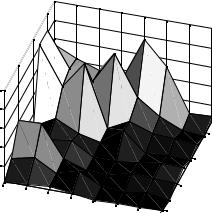
Figure 3.58 shows a macroblock from the original frame (taken from around the head of the figure on the right) and Figure 3.59 the luminance residual after motion compensation. Applying a 2D DCT to the top-right 8 × 8 block of luminance samples (Table 3.9) produces the DCT coefficients listed in Table 3.10. The magnitude of each coefficient is plotted in Figure 3.60; note that the larger coefficients are clustered around the top-left (DC) coefficient.
A simple forward quantiser is applied:
Qcoeff = round(coeff/Qstep)
where Qstep is the quantiser step size, 12 in this example. Small-valued coefficients become zero in the quantised block (Table 3.11) and the nonzero outputs are clustered around the top-left (DC) coefficient.
The quantised block is reordered in a zigzag scan (starting at the top-left) to produce a linear array:
−1, 2, 1, −1, −1, 2, 0, −1, 1, −1, 2, −1, −1, 0, 0, −1, 0, 0, 0, −1, −1, 0, 0, 0, 0, 0, 1, 0, . . .
THE HYBRID DPCM/DCT VIDEO CODEC MODEL |
|
|
|
79 |
|
|||||
|
|
|
|
|
|
|
|
|||
|
|
|
Table 3.10 DCT coefficients |
|
|
• |
||||
|
|
|
|
|
|
|
|
|
||
−13.50 |
20.47 |
20.20 |
2.14 |
−0.50 |
−10.48 |
−3.50 |
−0.62 |
|||
|
10.93 |
−11.58 |
−10.29 |
−5.17 |
−2.96 |
10.44 |
4.96 |
−1.26 |
|
|
|
−8.75 |
9.22 |
−17.19 |
2.26 |
3.83 |
−2.45 |
1.77 |
1.89 |
|
|
|
−7.10 |
−17.54 |
1.24 |
−0.91 |
0.47 |
−0.37 |
−3.55 |
0.88 |
|
|
19.00 |
−7.20 |
4.08 |
5.31 |
0.50 |
0.18 |
−0.61 |
0.40 |
|
|
|
−13.06 |
3.12 |
−2.04 −0.17 −1.19 |
1.57 |
−0.08 |
−0.51 |
|
|
|||
1.73 |
−0.69 |
1.77 |
0.78 |
−1.86 |
1.47 |
1.19 |
0.42 |
|
|
|
|
−1.99 |
−0.05 |
1.24 |
−0.48 |
−1.86 |
−1.17 |
−0.21 |
0.92 |
|
|
Table 3.11 Quantized coefficients
−1 |
2 |
2 |
0 |
0 |
−1 |
0 |
0 |
1 |
−1 |
−1 |
0 |
0 |
1 |
0 |
0 |
−1 |
1 |
−1 |
0 |
0 |
0 |
0 |
0 |
−1 |
−1 |
0 |
0 |
0 |
0 |
0 |
0 |
2 |
−1 |
0 |
0 |
0 |
0 |
0 |
0 |
−1 |
0 |
0 |
0 |
0 |
0 |
0 |
0 |
0 |
0 |
0 |
0 |
0 |
0 |
0 |
0 |
0 |
0 |
0 |
0 |
0 |
0 |
0 |
0 |
|
|
|
|
|
|
|
|
Figure 3.59 Residual macroblock (luminance)
This array is processed to produce a series of (zero run, level) pairs:
(0, −1)(0, 2)(0, 1)(0, −1)(0, −1)(0, 2)(1, −1)(0, 1)(0, −1)(0, 2)(0, −1)(0, −1)(2, −1)
(3, −1)(0, −1)(5, 1)(EOB)
‘EOB’ (End Of Block) indicates that the remainder of the coefficients are zero.
Each (run, level) pair is encoded as a VLC. Using the MPEG-4 Visual TCOEF table (Table 3.6), the VLCs shown in Table 3.12 are produced.
80 |
|
VIDEO CODING CONCEPTS |
||
|
|
|
|
|
• |
Table 3.12 Variable length coding example |
|||
|
|
|
||
Run, Level, Last |
VLC (including sign bit) |
|||
|
|
(0,−1, 0) |
101 |
|
|
|
(0,2, 0) |
11100 |
|
|
|
(0,1, 0) |
100 |
|
|
|
(0,−1, 0) |
101 |
|
|
|
(0,−1, 0) |
101 |
|
|
|
(0,2, 0) |
11100 |
|
|
|
(1,−1, 0) |
1101 |
|
|
|
· · · |
· · · |
|
|
|
(5,1, 1) |
00100110 |
|
25 |
|
|
|
|
|
|
|
|
20 |
|
|
|
|
|
|
|
|
15 |
|
|
|
|
|
|
|
|
10 |
|
|
|
|
|
|
|
2 |
|
|
|
|
|
|
|
|
|
5 |
|
|
|
|
|
|
|
4 |
1 |
2 |
3 |
|
|
|
|
|
6 |
|
4 |
|
|
|
|
|
||
|
|
5 |
|
|
|
|
||
|
|
|
6 |
|
|
|
||
|
|
|
|
7 |
|
8 |
||
|
|
|
|
|
8 |
|||
|
|
|
|
|
|
|||
|
|
|
|
|
|
|
|
Figure 3.60 DCT coefficient magnitudes (top-right 8 × 8 block)
The final VLC signals that LAST = 1, indicating that this is the end of the block. The motion vector for this macroblock is (0, 1) (i.e. the vector points downwards). The predicted vector (based on neighbouring macroblocks) is (0,0) and so the motion vector difference values are MVDx = 0, MVDy = +1. Using the MPEG4 MVD table (Table 3.7), these are coded as
(1) and (0010) respectively.
The macroblock is transmitted as a series of VLCs, including a macroblock header, motion vector difference (X and Y) and transform coefficients (TCOEF) for each 8 × 8 block.
At the decoder, the VLC sequence is decoded to extract header parameters, MVDx and MVDy and (run,level) pairs for each block. The 64-element array of reordered coefficients is reconstructed by inserting (run) zeros before every (level). The array is then ordered to produce an 8 × 8 block (identical to Table 3.11). The quantised coefficients are rescaled using:
Rcoeff = Qstep.Qcoeff
(where Qstep = 12 as before) to produce the block of coefficients shown in Table 3.13. Note that the block is significantly different from the original DCT coefficients (Table 3.10) due to
THE HYBRID DPCM/DCT VIDEO CODEC MODEL |
|
|
|
|
81 |
|
||||
|
|
|
|
|
|
|
||||
|
|
Table 3.13 Rescaled coefficients |
|
|
• |
|||||
|
|
|
|
|
|
|
|
|
||
|
−12 |
24 |
24 |
0 |
0 |
−12 |
0 |
0 |
||
12 |
−12 |
−12 |
0 |
0 |
12 |
0 |
0 |
|
|
|
|
−12 |
12 |
−12 |
0 |
0 |
0 |
0 |
0 |
|
|
|
−12 |
−12 |
0 |
0 |
0 |
0 |
0 |
0 |
|
|
24 |
−12 |
0 |
0 |
0 |
0 |
0 |
0 |
|
|
|
|
−12 |
0 |
0 |
0 |
0 |
0 |
0 |
0 |
|
|
0 |
0 |
0 |
0 |
0 |
0 |
0 |
0 |
|
|
|
0 |
0 |
0 |
0 |
0 |
0 |
0 |
0 |
|
|
|
|
|
|
|
|
|
|
|
|
|
|
Table 3.14 Decoded residual luminance samples
−3 −3 −1 |
1 |
−1 |
−1 |
−1 |
−3 |
||
5 |
3 |
2 |
0 |
−3 |
−4 |
−5 |
−6 |
9 |
6 |
1 |
−3 |
−5 |
−6 |
−5 |
−4 |
9 |
8 |
1 |
−4 |
−1 |
1 |
4 |
10 |
7 |
8 |
−1 |
−6 |
−1 |
2 |
5 |
14 |
2 |
3 |
−8 −15 −11 −11 −11 |
−2 |
||||
2 |
5 |
−7 |
−17 |
−13 |
−16 |
−20 |
−11 |
12 |
16 |
3 |
−6 |
−1 |
−6 −11 |
−3 |
|
Original residual block |
Decoded residual block |
20 |
|
|
20 |
|
0 |
|
0 |
0 |
0 |
|
2 |
|
|
2 |
-20 |
4 |
|
-20 |
4 |
0 |
|
0 |
||
|
|
|
||
2 |
6 |
|
2 |
6 |
4 |
|
4 |
||
|
|
|
||
6 |
8 |
|
6 |
8 |
8 |
|
8 |
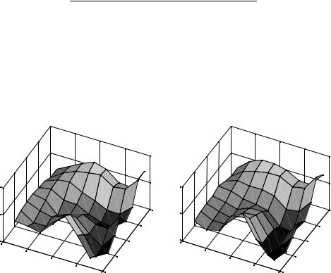
Figure 3.61 Comparison of original and decoded residual blocks
the quantisation process. An Inverse DCT is applied to create a decoded residual block (Table 3.14) which is similar but not identical to the original residual block (Table 3.9). The original and decoded residual blocks are plotted side by side in Figure 3.61 and it is clear that the decoded block has less high-frequency variation because of the loss of high-frequency DCT coefficients through quantisation.