

104 |
MPEG-4 VISUAL |
• |
video object |
VOP1 |
VOP2 |
VOP3 |
Time
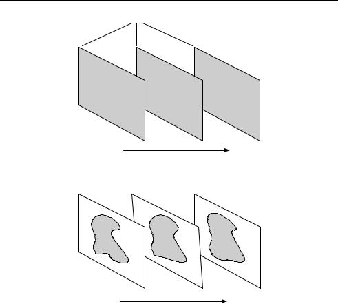
Figure 5.2 VOPs and VO (rectangular)
VOP1 |
VOP2 |
VOP3 |
|
||
|
|
Time
Figure 5.3 VOPs and VO (arbitrary shape)
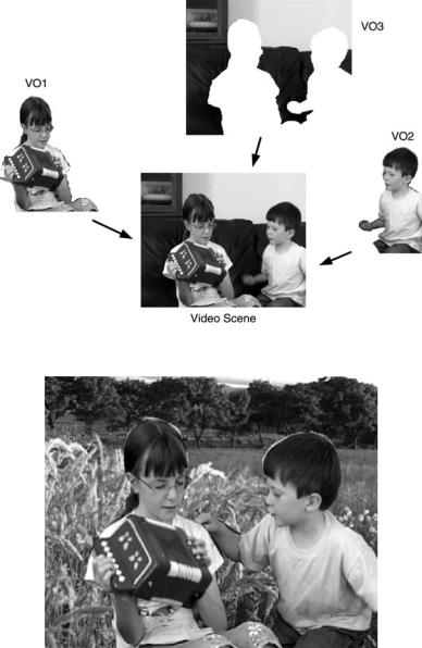
A video scene (e.g. Figure 5.4) may be made up of a background object (VO3 in this example) and a number of separate foreground objects (VO1, VO2). This approach is potentially much more flexible than the fixed, rectangular frame structure of earlier standards. The separate objects may be coded with different visual qualities and temporal resolutions to reflect their ‘importance’ to the final scene, objects from multiple sources (including synthetic and ‘natural’ objects) may be combined in a single scene and the composition and behaviour of the scene may be manipulated by an end-user in highly interactive applications. Figure 5.5 shows a new video scene formed by adding VO1 from Figure 5.4, a new VO2 and a new background VO. Each object is coded separately using MPEG-4 Visual (the compositing of visual and audio objects is assumed to be handled separately, for example by MPEG-4 Systems [2]).
5.3 CODING RECTANGULAR FRAMES
Notwithstanding the potential flexibility offered by object-based coding, the most popular application of MPEG-4 Visual is to encode complete frames of video. The tools required
CODING RECTANGULAR FRAMES |
• |
|
105 |
|
|
Figure 5.4 Video scene consisting of three VOs
Figure 5.5 Video scene composed of VOs from separate sources
to handle rectangular VOPs (typically complete video frames) are grouped together in the so-called simple profiles. The tools and objects for coding rectangular frames are shown in Figure 5.6. The basic tools are similar to those adopted by previous video coding standards, DCT-based coding of macroblocks with motion compensated prediction. The Simple profile is based around the well-known hybrid DPCM/DCT model (see Chapter 3, Section 3.6) with
106 |
MPEG-4 VISUAL |
|
• |
B-VOP |
|
Object |
Interlace |
|
Key: |
|
|
|
Alternate Quant |
|
Tool |
|
|
|
Global MC |
|
|
Quarter Pel |
|
I-VOP |
Advanced |
|
Simple |
||
P-VOP |
|
|
4MV |
|
|
UMV |
|
|
Intra Pred |
|
|
Video packets |
Simple |
|
|
||
Data Partitioning |
|
|
RVLCs |
Advanced Real |
|
|
||
|
Time Simple |
|
Short Header |
Dynamic |
|
Resolution |
||
|
||
|
Conversion |
|
|
NEWPRED |
|
Figure 5.6 Tools and objects for coding rectangular frames |
||
additional tools to improve coding efficiency and transmission efficiency. Because of the widespread popularity of Simple profile, enhanced profiles for rectangular VOPs have been developed. The Advanced Simple profile improves further coding efficiency and adds support for interlaced video and the Advanced Real-Time Simple profile adds tools that are useful for real-time video streaming applications.
5.3.1 Input and output video format
The input to an MPEG-4 Visual encoder and the output of a decoder is a video sequence in 4:2:0, 4:2:2 or 4:4:4 progressive or interlaced format (see Chapter 2). MPEG-4 Visual uses the sampling arrangement shown in Figure 2.11 for progressive sampled frames and the method shown in Figure 2.12 for allocating luma and chroma samples to each pair of fields in an interlaced sequence.
5.3.2 The Simple Profile
A CODEC that is compatible with Simple Profile should be capable of encoding and decoding Simple Video Objects using the following tools:
I-VOP (Intra-coded rectangular VOP, progressive video format);
P-VOP (Inter-coded rectangular VOP, progressive video format);
CODING RECTANGULAR FRAMES |
• |
|
107 |
|
|
source |
|
|
|
|
|
|
DCT |
|
|
|
Q |
|
|
|
Reorder |
|
|
|
|
RLE |
|
|
|
VLE |
|
|
|
|
|
|
|||||||||||||||||
frame |
|
|
|
|
|
|
|
|
|
|
|
|
|
|
|
|
|
|
|
|
|
|
|
|
|
||||||||||||||||||||||
|
|
|
|
|
|
|
|
|
|
|
|
|
|
|
|
|
|
|
|
|
|
|
|
|
|
|
|
|
|
|
|
|
|
|
|
|
|
|
|
|
|
|
|
|
|||
|
|
|
|
|
|
|
|
|
|
|
|
|
|
|
|
|
|
|
|
|
|
|
|
|
|
|
|
|
|
|
|
|
|
|
|
|
|
|
|
|
|
|
|
|
|
|
coded |
|
|
|
|
|
|
|
|
|
|
|
|
|
|
|
|
|
|
|
|
|
|
|
|
|
|
|
|
|
|
|
|
|
|
|
|
|
|
|
|
|
|
|
|
|
|
|
|
|
|
|
|
|
|
|
|
|
|
|
|
|
|
|
|
|
|
|
|
|
|
|
|
|
|
|
|
|
|
|
|
|
|
|
|
|
|
|
|
|
|
|
|
|
|
|
I-VOP |
decoded |
|
|
|
|
|
|
|
|
|
|
|
|
|
|
|
|
|
|
|
|
|
|
|
|
|
|
|
|
|
|
|
|
|
|
|
|
|
|
|
|
|
|
|
||||
|
|
|
|
|
|
IDCT |
|
|
|
Q-1 |
|
|
|
Reorder |
|
|
|
|
RLD |
|
|
|
VLD |
|
|
|
|
|
|
||||||||||||||||||
frame |
|
|
|
|
|
|
|
|
|
|
|
|
|
|
|
|
|
|
|
|
|
|
|
|
|||||||||||||||||||||||
|
|
|
|
|
|
|
|
|
|
|
|
|
|
|
|
|
|
|
|
|
|
|
|
|
|
|
|
|
|
|
|
|
|
|
|
|
|
|
|
|
|
|
|
|
|||
|
|
|
|
|
|
|
|
|
|
|
|
|
|
|
|
|
|
|
|
|
|
|
|
|
|
|
|
|
|
|
|
|
|
|
|
|
|
|
|
|
|
|
|
|
|
|
|
|
|
|
|
|
|
|
|
|
|
Figure 5.7 I-VOP encoding and decoding stages |
|||||||||||||||||||||||||||||||||||||
|
|
|
|
|
|
|
|
|
|
|
|
|
reconstructed |
|
|
|
|
|
|
|
|
|
|
|
|
|
|
|
|
|
|
|
|
|
|
|
|
||||||||||
|
|
|
|
|
|
ME |
|
|
|
|
|
|
|
|
|
|
|
|
|
|
|
|
|
|
|
|
|
|
|
|
|
|
|
||||||||||||||
|
|
|
|
|
|
|
|
|
|
|
|
frame |
|
|
|
|
|
|
|
|
|
|
|
|
|
|
|
|
|
|
|
|
|
|
|
|
|
|
|
||||||||
|
|
|
|
|
|
|
|
|
|
|
|
|
|
|
|
|
|
|
|
|
|
|
|
|
|
|
|
|
|
|
|
|
|
|
|
|
|
|
|
|
|
|
|||||
source |
|
|
|
|
|
|
|
|
|
|
|
|
|
|
|
|
|
|
|
|
|
|
|
|
|
|
|
|
|
|
|
|
|
|
|
|
|
|
|
|
|
|
|
|
|
|
|
|
|
|
|
|
|
|
|
|
|
|
|
|
|
|
|
|
|
|
|
|
|
|
|
|
|
|
|
|
|
|
|
|
|
|
|
|
|
|
|
|
|
|
|
|
|||
|
|
|
|
|
|
|
|
|
|
|
|
|
|
|
|
|
|
|
|
|
|
|
|
|
|
|
|
|
|
|
|
|
|
|
|
|
|
|
|
|
|
|
|
|
|||
|
|
|
MCP |
|
|
|
|
DCT |
|
|
|
|
|
Q |
|
|
|
|
Reorder |
|
|
|
RLE |
|
|
|
VLE |
|
|
|
|
||||||||||||||||
frame |
|
|
|
|
|
|
|
|
|
|
|
|
|
|
|
|
|
|
|
|
|
|
|
|
|
|
|||||||||||||||||||||
|
|
|
|
|
|
|
|
|
|
|
|
|
|
|
|
|
|
|
|
|
|
|
|
|
|
|
|
|
|
|
|
|
|
|
|
|
|
|
|
|
|
|
|
|
|||
|
|
|
|
|
|
|
|
|
|
|
|
|
|
|
|
|
|
|
|
|
|
|
|
|
|
|
|
|
|
|
|
|
|
|
|
|
|
|
|
|
|
|
|
|
|
|
coded |
|
|
|
|
|
|
|
|
|
|
|
|
|
|
|
|
|
|
|
|
|
|
|
|
|
|
|
|
|
|
|
|
|
|
|
|
|
|
|
|
|
|
|
|
|
|
|
P-VOP |
decoded |
|
|
|
|
|
|
|
|
|
|
|
|
|
|
|
|
|
|
|
|
|
|
|
|
|
|
|
|
|
|
|
|
|
|
|
|
|
|
|
|
|
|
|
|
|
|
|
|
|
|
MCR |
|
|
|
|
IDCT |
|
|
|
|
|
Q-1 |
|
|
|
|
Reorder |
|
|
|
RLD |
|
|
|
VLD |
|
|
|
|
||||||||||||||||
frame |
|
|
|
|
|
|
|
|
|
|
|
|
|
|
|
|
|
|
|
|
|
|
|
|
|
||||||||||||||||||||||
|
|
|
|
|
|
|
|
|
|
|
|
|
|
|
|
|
|
|
|
|
|
|
|
|
|
|
|
|
|
|
|
|
|
|
|
|
|
|
|
|
|
|
|
|
|||
Figure 5.8 P-VOP encoding and decoding stages
short header (mode for compatibility with H.263 CODECs);
compression efficiency tools (four motion vectors per macroblock, unrestricted motion vectors, Intra prediction);
transmission efficiency tools (video packets, Data Partitioning, Reversible Variable Length Codes).
5.3.2.1 The Very Low Bit Rate Video Core
The Simple Profile of MPEG-4 Visual uses a CODEC model known as the Very Low Bit Rate Video (VLBV) Core (the hybrid DPCM/DCT model described in Chapter 3). In common with other standards, the architecture of the encoder and decoder are not specified in MPEG-4 Visual but a practical implementation will require to carry out the functions shown in Figure 5.7 (coding of Intra VOPs) and Figure 5.8 (coding of Inter VOPs). The basic tools required to encode and decode rectangular I-VOPs and P-VOPs are described in the next section (Section 3.6 of Chapter 3 provides a more detailed ‘walk-through’ of the encoding and decoding process). The tools in the VLBV Core are based on the H.263 standard and the ‘short header’ mode enables direct compatibility (at the frame level) between an MPEG-4 Simple Profile CODEC and an H.263 Baseline CODEC.
5.3.2.2 Basic coding tools
I-VOP
A rectangular I-VOP is a frame of video encoded in Intra mode (without prediction from any other coded VOP). The encoding and decoding stages are shown in Figure 5.7.
108 |
|
|
|
|
MPEG-4 VISUAL |
||
|
|
|
|
||||
• |
Table 5.4 Values of dc scaler parameter depending on QP range |
||||||
|
|
|
|
|
|
||
Block type |
Q P ≤ 4 |
5 ≤ Q P ≤ 8 |
9 ≤ Q P ≤ 24 |
25 ≤ Q P |
|
||
|
|
Luma |
8 |
2 × Q P |
Q P + 8 |
(2 × Q P) − 16 |
|
|
|
Chroma |
8 |
(Q P + 13)/2 |
(Q P + 13)/2 |
Q P − 6 |
|
DCT and IDCT: Blocks of luma and chroma samples are transformed using an 8 × 8 Forward DCT during encoding and an 8 × 8 Inverse DCT during decoding (see Section 3.4).
Quantisation: The MPEG-4 Visual standard specifies the method of rescaling (‘inverse quantising’) quantised transform coefficients in a decoder. Rescaling is controlled by a quantiser scale parameter, QP, which can take values from 1 to 31 (larger values of QP produce a larger quantiser step size and therefore higher compression and distortion). Two methods of rescaling are described in the standard: ‘method 2’ (basic method) and ‘method 1’ (more flexible but also more complex). Method 2 inverse quantisation operates as follows. The DC coefficient in an Intra-coded macroblock is rescaled by:
DC = DCQ . dc scaler |
(5.1) |
DCQ is the quantised coefficient, DC is the rescaled coefficient and dc scaler is a parameter defined in the standard. In short header mode (see below), dc scaler is 8 (i.e. all Intra DC coefficients are rescaled by a factor of 8), otherwise dc scaler is calculated according to the value of QP (Table 5.4). All other transform coefficients (including AC and Inter DC) are rescaled as follows:
|F| = Q P · (2 · |FQ | + 1) |
(if QP is odd and FQ =0) |
|
|F| = Q P · (2 · |FQ | + 1) − 1 |
(if QP is even and FQ =0) |
(5.2) |
F = 0 |
(if FQ = 0) |
|
FQ is the quantised coefficient and F is the rescaled coefficient. The sign of F is made the same as the sign of FQ . Forward quantisation is not defined by the standard.
Zig-zag scan: Quantised DCT coefficients are reordered in a zig-zag scan prior to encoding (see Section 3.4).
Last-Run-Level coding: The array of reordered coefficients corresponding to each block is encoded to represent the zero coefficients efficiently. Each nonzero coefficient is encoded as a triplet of (last, run, level), where ‘last’ indicates whether this is the final nonzero coefficient in the block, ‘run’ signals the number of preceding zero coefficients and ‘level’ indicates the coefficient sign and magnitude.
Entropy coding: Header information and (last, run, level) triplets (see Section 3.5) are represented by variable-length codes (VLCs). These codes are similar to Huffman codes and are defined in the standard, based on pre-calculated coefficient probabilities
A coded I-VOP consists of a VOP header, optional video packet headers and coded macroblocks. Each macroblock is coded with a header (defining the macroblock type, identifying which blocks in the macroblock contain coded coefficients, signalling changes in quantisation parameter, etc.) followed by coded coefficients for each 8 × 8 block.
CODING RECTANGULAR FRAMES |
• |
|
109 |
|
|
In the decoder, the sequence of VLCs are decoded to extract the quantised transform coefficients which are re-scaled and transformed by an 8 × 8 IDCT to reconstruct the decoded I-VOP (Figure 5.7).
P-VOP
A P-VOP is coded with Inter prediction from a previously encoded I- or P-VOP (a reference VOP). The encoding and decoding stages are shown in Figure 5.8.
Motion estimation and compensation: The basic motion compensation scheme is blockbased compensation of 16 × 16 pixel macroblocks (see Chapter 3). The offset between the current macroblock and the compensation region in the reference picture (the motion vector) may have half-pixel resolution. Predicted samples at sub-pixel positions are calculated using bilinear interpolation between samples at integer-pixel positions. The method of motion estimation (choosing the ‘best’ motion vector) is left to the designer’s discretion. The matching region (or prediction) is subtracted from the current macroblock to produce a residual macroblock (Motion-Compensated Prediction, MCP in Figure 5.8).
After motion compensation, the residual data is transformed with the DCT, quantised, reordered, run-level coded and entropy coded. The quantised residual is rescaled and inverse transformed in the encoder in order to reconstruct a local copy of the decoded MB (for further motion compensated prediction). A coded P-VOP consists of VOP header, optional video packet headers and coded macroblocks each containing a header (this time including differentially-encoded motion vectors) and coded residual coefficients for every 8 × 8 block.
The decoder forms the same motion-compensated prediction based on the received motion vector and its own local copy of the reference VOP. The decoded residual data is added to the prediction to reconstruct a decoded macroblock (Motion-Compensated Reconstruction, MCR in Figure 5.8).
Macroblocks within a P-VOP may be coded in Inter mode (with motion compensated prediction from the reference VOP) or Intra mode (no motion compensated prediction). Inter mode will normally give the best coding efficiency but Intra mode may be useful in regions where there is not a good match in a previous VOP, such as a newly-uncovered region.
Short Header
The ‘short header’ tool provides compatibility between MPEG-4 Visual and the ITU-T H.263 video coding standard. An I- or P-VOP encoded in ‘short header’ mode has identical syntax to an I-picture or P-picture coded in the baseline mode of H.263. This means that an MPEG-4 I-VOP or P-VOP should be decodeable by an H.263 decoder and vice versa.
In short header mode, the macroblocks within a VOP are organised in Groups of Blocks (GOBs), each consisting of one or more complete rows of macroblocks. Each GOB may (optionally) start with a resynchronisation marker (a fixed-length binary code that enables a decoder to resynchronise when an error is encountered, see Section 5.3.2.4).
5.3.2.3 Coding Efficiency Tools
The following tools, part of the Simple profile, can improve compression efficiency. They are only used when short header mode is not enabled.

• |
MPEG-4 VISUAL |
110 |
Figure 5.9 One or four vectors per macroblock
Four motion vectors per macroblock
Motion compensation tends to be more effective with smaller block sizes. The default block size for motion compensation is 16 × 16 samples (luma), 8 × 8 samples (chroma), resulting in one motion vector per macroblock. This tool gives the encoder the option to choose a smaller motion compensation block size, 8 × 8 samples (luma) and 4 × 4 samples (chroma), giving four motion vectors per macroblock. This mode can be more effective at minimising the energy in the motion-compensated residual, particularly in areas of complex motion or near the boundaries of moving objects. There is an increased overhead in sending four motion vectors instead of one, and so the encoder may choose to send one or four motion vectors on a macroblock-by-macroblock basis (Figure 5.9).
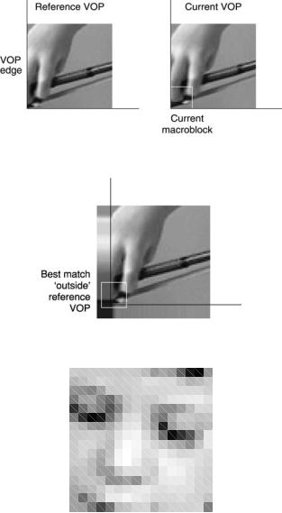
Unrestricted Motion Vectors
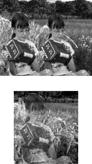
In some cases, the best match for a macroblock may be a 16 × 16 region that extends outside the boundaries of the reference VOP. Figure 5.10 shows the lower-left corner of a current VOP (right-hand image) and the previous, reference VOP (left-hand image). The hand holding the bow is moving into the picture in the current VOP and so there isn’t a good match for the highlighted macroblock inside the reference VOP. In Figure 5.11, the samples in the reference VOP have been extrapolated (‘padded’) beyond the boundaries of the VOP. A better match for the macroblock is obtained by allowing the motion vector to point into this extrapolated region (the highlighted macroblock in Figure 5.11 is the best match in this case). The Unrestricted Motion Vectors (UMV) tool allows motion vectors to point outside the boundary of the reference VOP. If a sample indicated by the motion vector is outside the reference VOP, the nearest edge sample is used instead. UMV mode can improve motion compensation efficiency, especially when there are objects moving in and out of the picture.
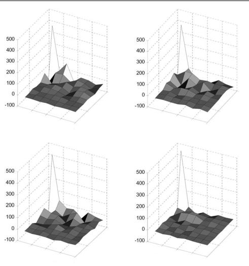
Intra Prediction
Low-frequency transform coefficients of neighbouring intra-coded 8 × 8 blocks are often correlated. In this mode, the DC coefficient and (optionally) the first row and column of AC coefficients in an Intra-coded 8 × 8 block are predicted from neighbouring coded blocks. Figure 5.12 shows a macroblock coded in intra mode and the DCT coefficients for each of the four 8 × 8 luma blocks are shown in Figure 5.13. The DC coefficients (top-left) are clearly
CODING RECTANGULAR FRAMES |
• |
|
111 |
|
|
Figure 5.10 Reference VOP and current VOP
Figure 5.11 Reference VOP extrapolated beyond boundary
Figure 5.12 Macroblock coded in intra mode
similar but it is less obvious whether there is correlation between the first row and column of the AC coefficients in these blocks.
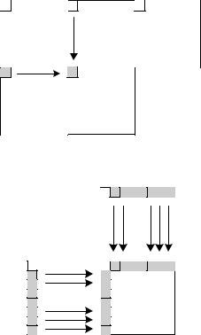
The DC coefficient of the current block (X in Figure 5.14) is predicted from the DC coefficient of the upper (C) or left (A) previously-coded 8 × 8 block. The rescaled DC coefficient values of blocks A, B and C determine the method of DC prediction. If A, B or C are outside the VOP boundary or the boundary of the current video packet (see later), or if they are not intra-coded, their DC coefficient value is assumed to be equal to
• |
MPEG-4 VISUAL |
112 |
500 |
|
|
|
500 |
|
|
400 |
|
|
|
400 |
|
|
300 |
|
|
|
300 |
|
|
200 |
|
|
|
200 |
|
|
100 |
|
|
|
100 |
|
|
0 |
|
|
0 |
0 |
|
0 |
-100 |
|
|
|
-100 |
|
|
0 |
|
|
|
|
|
|
5 |
|
0 |
5 |
|||
2 |
|
2 |
||||
|
|
4 |
|
|
|
4 |
|
|
6 |
|
|
|
6 |
|
|
8 |
|
|
|
8 |
|
|
Upper left |
|
|
|
Upper right |
500 |
|
|
|
500 |
|
|
400 |
|
|
|
400 |
|
|
300 |
|
|
|
300 |
|
|
200 |
|
|
|
200 |
|
|
100 |
|
|
|
100 |
|
|
0 |
|
0 |
|
0 |
|
0 |
|
|
|
|
|||
-100 |
|
|
|
-100 |
|
|
0 |
|
|
|
|
|
|
5 |
0 |
5 |
||||
2 |
2 |
|||||
|
|
4 |
|
|
|
4 |
|
|
6 |
|
|
|
6 |
|
|
8 |
|
|
|
8 |
|
|
Lower left |
|
|
|
Lower right |
Figure 5.13 DCT coefficients (luma blocks)
1024 (the DC coefficient of a mid-grey block of samples). The direction of prediction is determined by:
if |DCA − DCB| < |DCB − DCC| predict from block C
else
predict from block A
The direction of the smallest DC gradient is chosen as the prediction direction for block X. The prediction, PDC, is formed by dividing the DC coefficient of the chosen neighbouring
CODING RECTANGULAR FRAMES |
|
|
|
• |
|||
113 |
|
||||||
|
|
|
|
|
|
|
|
BC
AX
Figure 5.14 Prediction of DC coefficients
|
C |
A |
X |
Figure 5.15 Prediction of AC coefficients
block by a scaling factor and PDC is then subtracted from the actual quantised DC coefficient (QDCX) and the residual (PQDCX) is coded and transmitted.
AC coefficient prediction is carried out in a similar way, with the first row or column of AC coefficients predicted in the direction determined for the DC coefficient (Figure 5.15). For example, if the prediction direction is from block A, the first column of AC coefficients in block X is predicted from the first column of block A. If the prediction direction is from block C, the first row of AC coefficients in X is predicted from the first row of C. The prediction is scaled depending on the quantiser step sizes of blocks X and A or C.
5.3.2.4 Transmission Efficiency Tools
A transmission error such as a bit error or packet loss may cause a video decoder to lose synchronisation with the sequence of decoded VLCs. This can cause the decoder to decode incorrectly some or all of the information after the occurrence of the error and this means that part or all of the decoded VOP will be distorted or completely lost (i.e. the effect of the error spreads spatially through the VOP, ‘spatial error propagation’). If subsequent VOPs are predicted from the damaged VOP, the distorted area may be used as a prediction reference, leading to temporal error propagation in subsequent VOPs (Figure 5.16).

• |
MPEG-4 VISUAL |
114 |
error position
area damaged
forward prediction
Figure 5.16 Spatial and temporal error propagation
When an error occurs, a decoder can resume correct decoding upon reaching a resynchronisation point, typically a uniquely-decodeable binary code inserted in the bitstream. When the decoder detects an error (for example because an invalid VLC is decoded), a suitable recovery mechanism is to ‘scan’ the bitstream until a resynchronisation marker is detected. In short header mode, resynchronisation markers occur at the start of each VOP and (optionally) at the start of each GOB.
The following tools are designed to improve performance during transmission of coded video data and are particularly useful where there is a high probability of network errors [3]. The tools may not be used in short header mode.
Video Packet
A transmitted VOP consists of one or more video packets. A video packet is analogous to a slice in MPEG-1, MPEG-2 or H.264 (see Section 6) and consists of a resynchronisation marker, a header field and a series of coded macroblocks in raster scan order (Figure 5.17). (Confusingly, the MPEG-4 Visual standard occasionally refers to video packets as ‘slices’). The resynchronisation marker is followed by a count of the next macroblock number, which enables a decoder to position the first macroblock of the packet correctly. After this comes the quantisation parameter and a flag, HEC (Header Extension Code). If HEC is set to 1, it is followed by a duplicate of the current VOP header, increasing the amount of information that has to be transmitted but enabling a decoder to recover the VOP header if the first VOP header is corrupted by an error.
The video packet tool can assist in error recovery at the decoder in several ways, for example:
1. When an error is detected, the decoder can resynchronise at the start of the next video packet and so the error does not propagate beyond the boundary of the video packet.

CODING RECTANGULAR FRAMES |
• |
|
115 |
|
|
Sync |
Header |
HEC |
(Header) |
Macroblock data |
Sync |
|
|
|
|
|
|
Figure 5.17 Video packet structure
2.If used, the HEC field enables a decoder to recover a lost VOP header from elsewhere within the VOP.
3.Predictive coding (such as differential encoding of the quantisation parameter, prediction of motion vectors and intra DC/AC prediction) does not cross the boundary between video packets. This prevents (for example) an error in motion vector data from propagating to another video packet.
Data Partitioning
The data partitioning tool enables an encoder to reorganise the coded data within a video packet to reduce the impact of transmission errors. The packet is split into two partitions, the first (immediately after the video packet header) containing coding mode information for each macroblock together with DC coefficients of each block (for Intra macroblocks) or motion vectors (for Inter macroblocks). The remaining data (AC coefficients and DC coefficients of Inter macroblocks) are placed in the second partition following a resynchronisation marker. The information sent in the first partition is considered to be the most important for adequate decoding of the video packet. If the first partition is recovered, it is usually possible for the decoder to make a reasonable attempt at reconstructing the packet, even if the 2nd partition is damaged or lost due to transmission error(s).
Reversible VLCs
An optional set of Reversible Variable Length Codes (RVLCs) may be used to encode DCT coefficient data. As the name suggests, these codes can be correctly decoded in both the forward and reverse directions, making it possible for the decoder to minimise the picture area affected by an error.
A decoder first decodes each video packet in the forward direction and, if an error is detected (e.g. because the bitstream syntax is violated), the packet is decoded in the reverse direction from the next resynchronisation marker. Using this approach, the damage caused by an error may be limited to just one macroblock, making it easy to conceal the errored region. Figure 5.18 illustrates the use of error resilient decoding. The figure shows a video packet that uses HEC, data partitioning and RVLCs. An error occurs within the texture data and the decoder scans forward and backward to recover the texture data on either side of the error.
5.3.3 The Advanced Simple Profile
The Simple profile, introduced in the first version of the MPEG-4 Visual standard, rapidly became popular with developers because of its improved efficiency compared with previous standards (such as MPEG-1 and MPEG-2) and the ease of integrating it into existing video applications that use rectangular video frames. The Advanced Simple profile was incorporated
116 |
|
|
|
|
|
|
|
MPEG-4 VISUAL |
||
• |
|
Error |
|
|
||||||
|
|
|
|
|
|
|
|
|
|
|
|
|
|
|
|
|
|
|
|
|
|
|
Sync |
Header |
HEC |
Header + |
|
|
|
Texture |
Sync |
|
|
MV |
|
|
|
|
|||||
|
|
|
|
|
|
|
|
|
|
|
|
|
|
Decode in forward |
|
|
|
|
Decode in reverse |
||
|
|
|
|
|
|
|
||||
|
|
|
|
|
|
|
||||
|
|
|
|
direction |
|
|
|
|
direction |
|
Figure 5.18 Error recovery using RVLCs
into a later version of the standard with added tools to support improved compression efficiency and interlaced video coding. An Advanced Simple Profile CODEC must be capable of decoding Simple objects as well as Advanced Simple objects which may use the following tools in addition to the Simple Profile tools:
B-VOP (bidirectionally predicted Inter-coded VOP);
quarter-pixel motion compensation;
global motion compensation;
alternate quantiser;
interlace (tools for coding interlaced video sequences).
B-VOP
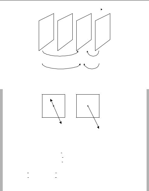
The B-VOP uses bidirectional prediction to improve motion compensation efficiency. Each block or macroblock may be predicted using (a) forward prediction from the previous I- or P-VOP, (b) backwards prediction from the next I- or P-VOP or (c) an average of the forward and backward predictions. This mode generally gives better coding efficiency than basic forward prediction; however, the encoder must store multiple frames prior to coding each B-VOP which increases the memory requirements and the encoding delay. Each macroblock in a B-VOP is motion compensated from the previous and/or next I- or P-VOP in one of the following ways (Figure 5.19).
1.Forward prediction: A single MV is transmitted, MVF, referring to the previous I- or P-VOP.
2.Backward prediction: A single MV is transmitted, MVB, referring to the future I- or P-VOP.
3.Bidirectional interpolated prediction: Two MVs are transmitted, MVF and MVB, referring to the previous and the future I- or P-VOPs. The motion compensated prediction for the current macroblock is produced by interpolating between the luma and chroma samples in the two reference regions.
4.Bidirectional direct prediction: Motion vectors pointing to the previous and future I- or P-VOPs are derived automatically from the MV of the same macroblock in the future I- or P-VOP. A ‘delta MV’ correcting these automatically-calculated MVs is transmitted.
CODING RECTANGULAR FRAMES |
117 |
|
|
temporal order |
• |
I B B P
Forward |
Backward |
Bidirectional
Figure 5.19 Prediction modes for B-VOP
MB in B6 |
MB in P7 |
MVB
MVF |
MVF |
Figure 5.20 Direct mode vectors
Example of direct mode (Figure 5.20)
Previous reference VOP: |
I4 , display time = 2 |
Current B-VOP: |
B6 , display time = 6 |
Future reference VOP: |
P7 , display time = 7 |
MV for same macroblock position in P7 , MV7 = (+5, −10)
TRB = display time(B6 ) – display time(I4 ) = 4
TRD = display time(P7 ) – display time(I4 ) = 5
MVD = 0 (no delta vector)
MVF = (TRB/TRD).MV = (+4, −8)
MVB = (TRB-TRD/TRD).MV = (−1, +2)
Quarter-Pixel Motion Vectors
The Simple Profile supports motion vectors with half-pixel accuracy and this tool supports vectors with quarter-pixel accuracy. The reference VOP samples are interpolated to half-pixel positions and then again to quarter-pixel positions prior to motion estimation and compensation. This increases the complexity of motion estimation, compensation and reconstruction
118 |
|
|
|
|
|
|
|
MPEG-4 VISUAL |
||
|
|
|
|
|
|
|
|
|||
• |
|
|
Table 5.5 Weighting matrix W |
|
|
|
||||
|
|
|
|
|
w |
|
|
|
||
10 |
20 |
20 |
30 |
30 |
30 |
40 |
40 |
|
||
|
|
20 |
20 |
30 |
30 |
30 |
40 |
40 |
40 |
|
|
|
20 |
30 |
30 |
30 |
40 |
40 |
40 |
40 |
|
|
|
30 |
30 |
30 |
30 |
40 |
40 |
40 |
50 |
|
|
|
30 |
30 |
30 |
40 |
40 |
40 |
50 |
50 |
|
|
|
30 |
40 |
40 |
40 |
40 |
40 |
50 |
50 |
|
|
|
40 |
40 |
40 |
40 |
50 |
50 |
50 |
50 |
|
|
|
40 |
40 |
40 |
50 |
50 |
50 |
50 |
50 |
|
|
|
|
|
|
|
|
|
|
|
|
but can provide a gain in coding efficiency compared with half-pixel compensation (see Chapter 3).
Alternate quantiser
An alternative rescaling (‘inverse quantisation’) method is supported in the Advanced Simple Profile. Intra DC rescaling remains the same (see Section 5.3.2) but other quantised coefficients may be rescaled using an alternative method1.
Quantised coefficients FQ(u, v) are rescaled to produce coefficients F(u, v) (where u, vare the coordinates of the coefficient) as follows:
F = 0 |
if FQ = 0 |
(5.3) |
F = [(2.FQ(u, v) + k) · Ww(u, v) · Q P]/16 |
if FQ =0 |
|
0intra blocks
k = +1 FQ(u, v) > 0, nonintra−1 Fr m Q (u, v) < 0, nonintra
where WW is a matrix of weighting factors, W0 for intra macroblocks and W1 for nonintra macroblocks. In Method 2 rescaling (see Section 5.3.2.1), all coefficients (apart from Intra DC) are quantised and rescaled with the same quantiser step size. Method 1 rescaling allows an encoder to vary the step size depending on the position of the coefficient, using the weighting matrix WW. For example, better subjective performance may be achieved by increasing the step size for high-frequency coefficients and reducing it for low-frequency coefficients. Table 5.5 shows a simple example of a weighting matrix WW.
Global Motion Compensation
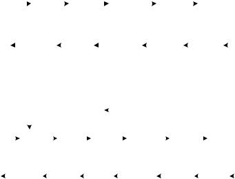
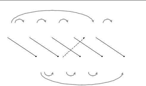
Macroblocks within the same video object may experience similar motion. For example, camera pan will produce apparent linear movement of the entire scene, camera zoom or rotation will produce a more complex apparent motion and macroblocks within a large object may all move in the same direction. Global Motion Compensation (GMC) enables an encoder to transmit a small number of motion (warping) parameters that describe a default ‘global’ motion for the entire VOP. GMC can provide improved compression efficiency when a significant number of macroblocks in the VOP share the same motion characteristics. The global motion
1 The MPEG-4 Visual standard describes the default rescaling method as ‘Second Inverse Quantisation Method’ and the alternative, optional method as ‘First Inverse Quantisation Method’. The default (‘Second’) method is sometimes known as ‘H.263 quantisation’ and the alternative (‘First’) method as ‘MPEG-4 quantisation’.

CODING RECTANGULAR FRAMES |
• |
|
119 |
|
|
Global MV
Interpolated MV |
Figure 5.21 VOP, GMVs and interpolated vector
Figure 5.22 GMC (compensating for rotation)
parameters are encoded in the VOP header and the encoder chooses either the default GMC parameters or an individual motion vector for each macroblock.
When the GMC tool is used, the encoder sends up to four global motion vectors (GMVs) for each VOP together with the location of each GMV in the VOP. For each pixel position in the VOP, an individual motion vector is calculated by interpolating between the GMVs and the pixel position is motion compensated according to this interpolated vector (Figure 5.21). This mechanism enables compensation for a variety of types of motion including rotation (Figure 5.22), camera zoom (Figure 5.23) and warping as well as translational or linear motion.
The use of GMC is enabled by setting the parameter sprite enable to ‘GMC’ in a Video Object Layer (VOL) header. VOPs in the VOL may thereafter be coded as S(GMC)-VOPs (‘sprite’ VOPs with GMC), as an alternative to the ‘usual’ coding methods (I-VOP, P-VOP or B-VOP). The term ‘sprite’ is used here because a type of global motion compensation is applied in the older ‘sprite coding’ mode (part of the Main Profile, see Section 5.4.2.2).
• |
MPEG-4 VISUAL |
120 |
Figure 5.23 GMC (compensating for camera zoom)
Figure 5.24 Close-up of interlaced VOP
Interlace
Interlaced video consists of two fields per frame (see Chapter 2) sampled at different times (typically at 50 Hz or 60 Hz temporal sampling rate). An interlaced VOP contains alternate lines of samples from two fields. Because the fields are sampled at different times, horizontal movement may reduce correlation between lines of samples (for example, in the moving face in Figure 5.24). The encoder may choose to encode the macroblock in Frame DCT mode, in which each block is transformed as usual, or in Field DCT mode, in which the luminance samples from Field 1 are placed in the top eight lines of the macroblock and the samples from Field 2 in the lower eight lines of the macroblock before calculating the DCT (Figure 5.25). Field DCT mode gives better performance when the two fields are decorrelated.
In Field Motion Compensation mode (similar to 16 × 8 Motion Compensation Mode in the MPEG-two standard), samples belonging to the two fields in a macroblock are motion
CODING RECTANGULAR FRAMES |
• |
|
121 |
|
|
. |
. |
. |
Figure 5.25 Field DCT
compensated separately so that two motion vectors are generated for the macroblock, one for the first field and one for the second. The Direct Mode used in B-VOPs (see above) is modified to deal with macroblocks that have Field Motion Compensated reference blocks. Two forward and two backward motion vectors are generated, one from each field in the forward and backward directions. If the interlaced video tool is used in conjunction with object-based coding (see Section 5.4), the padding process may be applied separately to the two fields of a boundary macroblock.
5.3.4 The Advanced Real Time Simple Profile
Streaming video applications for networks such as the Internet require good compression and error-robust video coding tools that can adapt to changing network conditions. The coding and error resilience tools within Simple Profile are useful for real-time streaming applications and the Advanced Real Time Simple (ARTS) object type adds further tools to improve error resilience and coding flexibility, NEWPRED (multiple prediction references) and Dynamic Resolution Conversion (also known as Reduced Resolution Update). An ARTS Profile CODEC should support Simple and ARTS object types.
NEWPRED
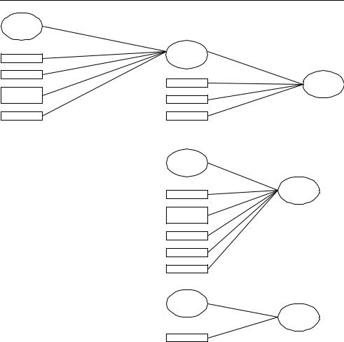
The NEWPRED (‘new prediction’) tool enables an encoder to select a prediction reference VOP from any of a set of previously encoded VOPs for each video packet. A transmission error that is imperfectly concealed will tend to propagate temporally through subsequent predicted VOPs and NEWPRED can be used to limit temporal propagation as follows (Figure 5.26). Upon detecting an error in a decoded VOP (VOP1 in Figure 5.26), the decoder sends a feedback message to the encoder identifying the errored video packet. The encoder chooses a reference VOP prior to the errored packet (VOP 0 in this example) for encoding of the following VOP (frame 4). This has the effect of ‘cleaning up’ the error and halting temporal propagation. Using NEWPRED in this way requires both encoder and decoder to store multiple reconstructed VOPs to use as possible prediction references. Predicting from an older reference VOP (4 VOPs in the past in this example) tends to reduce compression performance because the correlation between VOPs reduces with increasing time.
• |
MPEG-4 VISUAL |
122 |
Encoder
predict from older reference VOP
0 |
|
1 |
|
2 |
|
3 |
|
4 |
|
5 |
|
|
|
|
|
|
|
|
|
|
|
feedback indication
0 |
|
1 |
|
2 |
|
3 |
|
4 |
||||||||||
|
|
|
|
|
|
|
|
|
|
|
|
|
|
|
|
|
|
|
|
|
|
|
|
|
|
|
|
|
|
|
|
|
|
|
|
|
|
|
|
|
|
|
|
|
|
|
|
|
|
|
|
|
|
|
|
|
initial error
Decoder
predict from older reference VOP
Figure 5.26 NEWPRED error handling
Dynamic Resolution Conversion
Dynamic Resolution Conversion (DRC), otherwise known as Reduced Resolution (RR) mode, enables an encoder to encode a VOP with reduced spatial resolution. This can be a useful tool to prevent sudden increases in coded bitrate due to (for example) increased detail or rapid motion in the scene. Normally, such a change in the scene content would cause the encoder to generate a large number of coded bits, causing problems for a video application transmitting over a limited bitrate channel. Using the DRC tool, a VOP is encoded at half the normal horizontal and vertical resolution. At the decoder, a residual macroblock within a Reduced Resolution VOP is decoded and upsampled (interpolated) so that each 8 × 8 luma block covers an area of 16 × 16 samples. The upsampled macroblock (now covering an area of 32 × 32 luma samples) is motion compensated from a 32 × 32-sample reference area (the motion vector of the decoded macroblock is scaled up by a factor of 2) (Figure 5.27). The result is that the Reduced Resolution VOP is decoded at half the normal resolution (so that the VOP detail is reduced) with the benefit that the coded VOP requires fewer bits to transmit than a full-resolution VOP.
5.4 CODING ARBITRARY-SHAPED REGIONS
Coding objects of arbitrary shape (see Section 5.2.3) requires a number of extensions to the block-based VLBV core CODEC [4]. Each VOP is coded using motion compensated prediction and DCT-based coding of the residual, with extensions to deal with the special cases introduced by object boundaries. In particular, it is necessary to deal with shape coding, motion compensation and texture coding of arbitrary-shaped video objects.
32 |
• |
|
CODING ARBITRARY-SHAPED REGIONS |
123 |
|
16
8 |
upsample |
|
|
16 Y |
|
Y |
16 |
Cr Cb 8 |
32 |
|
|
motion compensate
16
Cr Cb
decoded macroblock
32
Y16
32
16
Cr Cb
32x32 sample reference area
Figure 5.27 Reduced Resolution decoding of a macroblock
Shape coding: The shape of a video object is defined by Alpha Blocks, each covering a 16 × 16-pixel area of the video scene. Each Alpha Block may be entirely external to the video object (in which case nothing needs to be coded), entirely internal to the VO (in which case the macroblock is encoded as in Simple Profile) or it may cross a boundary of the VO. In this last case, it is necessary to define the shape of the VO edge within the Alpha Block. Shape information is defined using the concept of ‘transparency’, where a ‘transparent’ pixel is not part of the current VOP, an ‘opaque’ pixel is part of the VOP and replaces anything ‘underneath’ it and a ‘semi-transparent’ pixel is part of the VOP and is partly transparent. The shape information may be defined as binary (all pixels are either opaque, 1, or transparent, 0) or grey scale (a pixel’s transparency is defined by a number between 0, transparent, and 255, opaque). Binary shape information for a boundary macroblock is coded as a binary alpha block (BAB) using arithmetic coding and grey scale shape information is coded using motion compensation and DCT-based encoding.
Motion compensation: Each VOP may be encoded as an I-VOP (no motion compensation), a P-VOP (motion compensated prediction from a past VOP) or a B-VOP (bidirection motion compensated prediction). Nontransparent pixels in a boundary macroblock are motion compensated from the appropriate reference VOP(s) and the boundary pixels of a reference
• |
MPEG-4 VISUAL |
124 |
Simple
B-VOP
Binary shape
PVOP temporal scalability
Alternate Quant
Core
Gray shape
Interlace
Sprite
Core
Quarter pel
Shape adaptive DCT
Global MC
Gray shape
Interlace
Core
N-Bit
Main
Advanced
Coding
Efficiency
N-Bit
Figure 5.28 Tools and objects for coding arbitrary-shaped regions
VOP are ‘padded’ to the edges of the motion estimation search area to fill the transparent pixel positions with data.
Texture coding: Motion-compensated residual samples (‘texture’) in internal blocks are coded using the 8 × 8 DCT, quantisation and variable length coding described in Section 5.3.2.1. Non-transparent pixels in a boundary block are padded to the edge of the 8 × 8 block prior to applying the DCT.
Video object coding is supported by the Core and Main profiles, with extra tools in the Advanced Coding Efficiency and N-Bit profiles (Figure 5.28).
5.4.1 The Core Profile
A Core Profile CODEC should be capable of encoding and decoding Simple Video Objects and Core Video Objects. A Core VO may use any of the Simple Profile tools plus the following:
CODING ARBITRARY-SHAPED REGIONS |
• |
|
125 |
|
|
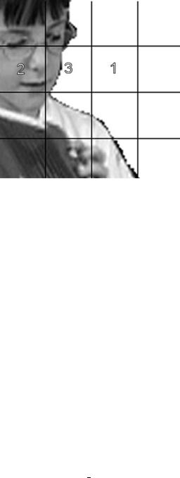
Figure 5.29 VO showing external (1), internal (2) and boundary (3) macroblocks
B-VOP (described in Section 5.3.3);
alternate quantiser (described in Section 5.3.3);
object-based coding (with Binary Shape);
P-VOP temporal scalability.
Scalable coding, described in detail in Section 5.5, enables a video sequence to be coded and transmitted as two or more separate ‘layers’ which can be decoded and re-combined. The Core Profile supports temporal scalability using P-VOPs and an encoder using this tool can transmit two coded layers, a base layer (decodeable as a low frame-rate version of the video scene) and a temporal enhancement layer containing only P-VOPs. A decoder can increase the frame rate of the base layer by adding the decoded frames from the enhancement layer.
Probably the most important functionality in the Core Profile is its support for coding of arbitrary-shaped objects, requiring several new tools. Each macroblock position in the picture is classed as (1) opaque (fully ‘inside’ the VOP), (2) transparent (not part of the VOP) or (3) on the boundary of the VOP (Figure 5.29).
In order to indicate the shape of the VOP to the decoder, alpha mask information is sent for every macroblock. In the Core Profile, only binary alpha information is permitted and each pixel position in the VOP is defined to be completely opaque or completely transparent. The Core Profile supports coding of binary alpha information and provides tools to deal with the special cases of motion and texture coding within boundary macroblocks.
5.4.1.1 Binary Shape Coding
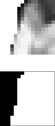
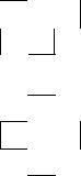
For each macroblock in the picture, a code bab type is transmitted. This code indicates whether the MB is transparent (not part of the current VOP, therefore no further data should be coded), opaque (internal to the current VOP, therefore motion and texture are coded as usual) or a boundary MB (part of the MB is opaque and part is transparent). Figure 5.30 shows a video object plane and Figure 5.31 is the corresponding binary mask indicating which pixels are
• |
MPEG-4 VISUAL |
126 |
Figure 5.30 VOP
Figure 5.31 Binary alpha mask (complete VOP)
part of the VOP (white) and which pixels are outside the VOP (black). For a boundary MB (e.g. Figure 5.32), it is necessary to encode a binary alpha mask to indicate which pixels are transparent and which are opaque (Figure 5.33).
The binary alpha mask (BAB) for each boundary macroblock is coded using Contextbased binary Arithmetic Encoding (CAE). A BAB pixel value X is to be encoded, where X is either 0 or 1. First, a context is calculated for the current pixel. A context template defines a region of n neighbouring pixels that have previously been coded (spatial neighbours for intracoded BABs, spatial and temporal neighbours for inter-coded BABs). The n values of each
CODING ARBITRARY-SHAPED REGIONS |
• |
||
127 |
|
||
|
|
|
|
Figure 5.32 Boundary macroblock
Figure 5.33 Binary alpha mask (boundary MB)
BAB pixel in the context form an n-bit word, the context for pixel X. There are 2n possible contexts and P(0), the probability that X is 0 given a particular context, is stored in the encoder and decoder for each possible n-bit context. Each mask pixel X is coded as follows:
1.Calculate the context for X.
2.Look up the relevant entry in the probability table P(0).
3.Encode X with an arithmetic encoder (see Chapter 3 for an overview of arithmetic coding). The sub-range is 0 . . . P(0) if X is 0 (black), P(0) . . . 1.0 if X is 1 (white).
Intra BAB Encoding
In an intra-coded BAB, the context template for the current mask pixel is formed from 10 spatially neighbouring pixels that have been previously encoded, c0 to c9 in Figure 5.34. The context is formed from the 10-bit word c9c8c7c6c5c4c3c2c1c0. Each of the 1024 possible context probabilities is listed in a table in the MPEG-4 Visual standard as an integer in the range 0 to 65535 and the actual probability of zero P(0) is derived by dividing this integer by 65535.

• |
MPEG-4 VISUAL |
128 |
c9 c8 c7
c6 |
c5 |
c4 |
c3 |
c2 |
c1 |
c0 |
X |
|
|
Figure 5.34 Context template for intra BAB
Examples
Context (binary) |
Context (decimal) |
Description |
P(0) |
|
|
|
|
0000000000 |
0 |
All context pixels are 0 |
65267/65535 = 0.9959 |
0000000001 |
1 |
c0 is 1, all others are 0 |
16468/65535 = 0.2513 |
1111111111 |
1023 |
All context pixels are 1 |
235/65535 = 0.0036 |
The context template (Figure 5.34) extends 2 pixels horizontally and vertically from the position of X. If any of these pixels are undefined (e.g. c2, c3 and c7 may be part of a BAB that has not yet been coded, or some of the pixels may belong to transparent BABs), the undefined pixels are set to the value of the nearest neighbour within the current BAB. Depending on the shape of the binary mask, more efficient coding may be obtained by scanning through the BAB in vertical order (rather than raster order) so that the context template is placed on its ‘side’. The choice of scan order for each BAB is signalled in the bitstream.
Inter BAB Encoding
The context template (Figure 5.35) consists of nine pixel positions, four in the current VOP (c0 to c3) and five in a reference VOP (c4 to c8). The position of the central context pixel in the reference VOP (c6) may be offset from the position X by an integer sample vector, enabling an inter BAB to be encoded using motion compensation. This ‘shape’ vector (MVs) may be chosen independently of any ‘texture’ motion vector. There are nine context pixels and so a total of 29 = 512 probabilities P(0) are stored by the encoder and decoder.
Examples:
Context (binary) |
Context (decimal) |
Description |
P(0) |
|
|
|
|
000000001 |
1 |
c0 is 1, all others 0 |
62970/65535 = 0.9609 |
000100000 |
64 |
c6 is 1, all others 0 |
23130/65535 = 0.3529 |
000100001 |
65 |
c6 and c0 are 1, all others 0 |
7282/65535 = 0.1111 |
These examples indicate that the transparency of the current pixel position X is more heavily influenced by c6 (the same position in the previous motion-compensated BAB) than c0 (the previous pixel position in raster scan order). As with intra-coding, the scanning order of the current (and previous) BAB may be horizontal or vertical.
CODING ARBITRARY-SHAPED REGIONS |
• |
|
129 |
|
|
c3 c2 c1
c0 X
c8
c7 c6 c5
c4
Figure 5.35 Context template for inter BAB
A single vector MVs is coded for each boundary inter-coded BAB. For P-VOPs, the reference VOP is the previous I- or P-VOP and for a B-VOP, the reference VOP is the temporally ‘nearest’ I- or P-VOP.
5.4.1.2 Motion Compensated Coding of Arbitrary-shaped VOPs
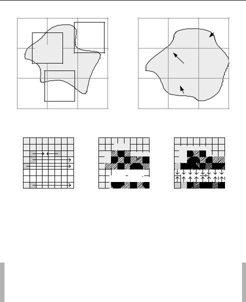
A P-VOP or B-VOP is predicted from a reference I- or P-VOP using motion compensation. It is possible for a motion vector to point to a reference region that extends outside of the opaque area of the reference VOP, i.e. some of the pixels in the reference region may be ‘transparent’. Figure 5.36 illustrates three examples. The left-hand diagram shows a reference VOP (with opaque pixels coloured grey) and the right-hand diagram shows a current VOP consisting of nine macroblocks. MB1 is entirely opaque but its MV points to a region in the reference VOP that contains transparent pixels. MB2 is a boundary MB and the opaque part of its motion-compensated reference region is smaller than the opaque part of MB2. MB3 is also a boundary MB and part of its reference region is located in a completely transparent MB in the reference VOP. In each of these cases, some of the opaque pixels in the current MB are motioncompensated from transparent pixels in the reference VOP. The values of transparent pixels are not defined and so it is necessary to deal with these special cases. This is done by padding transparent pixel positions in boundary and transparent macroblocks in the reference VOP.
Padding of Boundary MBs
Transparent pixels in each boundary MB in a reference VOP are extrapolated horizontally and vertically from opaque pixels as shown in Figure 5.37.
1.Opaque pixels at the edge of the BAB (dark grey in Figure 5.37) are extrapolated horizontally to fill transparent pixel positions in the same row. If a row is bordered by opaque pixels at only one side, the value of the nearest opaque pixel is copied to all transparent pixel positions. If a row is bordered on two sides by opaque pixels (e.g. the top row in Figure 5.37(a)), the transparent pixel positions are filled with the mean value of the two neighbouring opaque pixels. The result of horizontal padding is shown in Figure 5.37(b).
2.Opaque pixels (including those ‘filled’ by the first stage of horizontal padding) are extrapolated vertically to fill the remaining transparent pixel positions. Columns of transparent
• |
MPEG-4 VISUAL |
130 |
Reference VOP
Reference |
area for |
MB3 |
Reference |
area for |
MB1 |
Reference |
area for |
MB2 |
Current VOP
MB3 |
MB1 |
MB2 |
Figure 5.36 Examples of reference areas containing transparent pixels
(a) Horizontal padding |
(b) After horizontal padding |
(c) Vertical padding |
Figure 5.37 Horizontal and vertical padding in boundary MB
pixels with one opaque neighbour are filled with the value of that pixel and columns with two opaque neighbours (such as those in Figure 5.37(c)) are filled with the mean value of the opaque pixels at the top and bottom of the column.
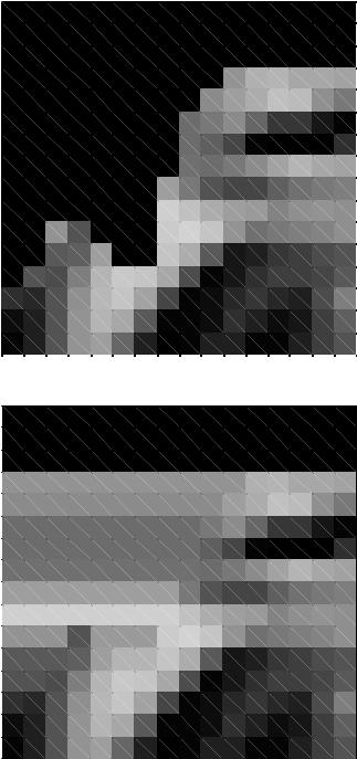
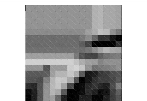
Example
Figure 5.38 shows a boundary macroblock from a VOP with transparent pixels plotted in black. The opaque pixels are extrapolated horizontally (step 1) to produce Figure 5.39 (note that five transparent pixel positions have two opaque horizontal neighbours). The result of step 1 is then extrapolated vertically (step 2) to produce Figure 5.40.
Padding of Transparent MBs
Fully transparent MBs must also be filled with padded pixel values because they may fall partly or wholly within a motion-compensated reference region (e.g. the reference region for MB3 in Figure 5.36). Transparent MBs with a single neighbouring boundary MB are filled by horizontal or vertical extrapolation of the boundary pixels of that MB. For example, in Figure 5.41, a transparent MB to the left of the boundary MB shown in Figure 5.38 is padded by filling each pixel position in the transparent MB with the value of the horizontally adjacent
CODING ARBITRARY-SHAPED REGIONS |
• |
|||||||||||||||||
131 |
|
|||||||||||||||||
|
|
|
|
|
|
|
|
|
|
|
|
|
|
|
|
|
|
|
|
|
|
|
|
|
|
|
|
|
|
|
|
|
|
|
|
|
|
|
|
|
|
|
|
|
|
|
|
|
|
|
|
|
|
|
|
|
|
|
|
|
|
|
|
|
|
|
|
|
|
|
|
|
|
|
|
|
|
|
|
|
|
|
|
|
|
|
|
|
|
|
|
|
|
|
|
|
|
|
|
|
|
|
|
|
|
|
|
|
|
|
|
|
|
|
|
|
|
|
|
|
|
|
|
|
|
|
|
|
|
|
|
|
|
|
|
|
|
|
|
|
|
|
|
|
|
|
|
|
|
|
|
|
|
|
|
|
|
|
|
|
|
|
|
|
|
|
|
|
|
|
|
|
|
|
|
|
|
|
|
|
|
|
|
|
|
|
|
|
|
|
|
|
|
|
|
|
|
|
|
|
|
|
|
|
|
|
|
|
|
|
|
|
|
|
|
|
|
|
|
|
|
|
|
|
|
|
|
|
|
|
|
|
|
|
|
|
|
|
|
|
|
|
|
|
|
|
|
|
|
|
|
|
|
|
|
|
|
|
|
|
|
|
|
|
|
|
|
|
|
|
|
|
|
|
|
|
|
|
|
|
|
|
|
|
|
|
|
|
|
|
|
|
|
|
|
|
|
|
|
|
|
|
|
|
|
|
|
|
|
|
|
|
|
|
|
|
|
|
|
|
|
|
Figure 5.38 Boundary MB
Figure 5.39 Boundary MB after horizontal padding
• |
MPEG-4 VISUAL |
132 |
Figure 5.40 Boundary MB after vertical padding
edge pixel. Transparent MBs are always padded after all boundary MBs have been fully padded.
If a transparent MB has more than one neighbouring boundary MB, one of its neighbours is chosen for extrapolation according to the following rule. If the left-hand MB is a boundary MB, it is chosen; else if the top MB is a boundary MB, it is chosen; else if the right-hand MB is a boundary MB, it is chosen; else the lower MB is chosen.
Transparent MBs with no nontransparent neighbours are filled with the pixel value 2N −1, where N is the number of bits per pixel. If N is 8 (the usual case), these MBs are filled with the pixel value 128.
5.4.1.3 Texture Coding in Boundary Macroblocks
The texture in an opaque MB (the pixel values in an intra-coded MB or the motion compensated residual in an inter-coded MB) is coded by the usual process of 8 × 8 DCT, quantisation, runlevel encoding and entropy encoding (see Section 5.3.2). A boundary MB consists partly of texture pixels (inside the boundary) and partly of undefined, transparent pixels (outside the boundary). In a core profile object, each 8 × 8 texture block within a boundary MB is coded using an 8 × 8 DCT followed by quantisation, run-level coding and entropy coding as usual (see Section 7.2 for an example). (The Shape-Adaptive DCT, part of the Advanced Coding Efficiency Profile and described in Section 5.4.3, provides a more efficient method of coding boundary texture.)

CODING ARBITRARY-SHAPED REGIONS |
133 |
|
• |
Figure 5.41 Padding of transparent MB from horizontal neighbour
5.4.2 The Main Profile
A Main Profile CODEC supports Simple and Core objects plus Scalable Texture objects (see Section 5.6.1) and Main objects. The Main object adds the following tools:
interlace (described in Section 5.3.3);
object-based coding with grey (‘alpha plane’) shape;
Sprite coding.
In the Core Profile, object shape is specified by a binary alpha mask such that each pixel position is marked as ‘opaque’ or ‘transparent’. The Main Profile adds support for grey shape masks, in which each pixel position can take varying levels of transparency from fully transparent to fully opaque. This is similar to the concept of Alpha Planes used in computer graphics and allows the overlay of multiple semi-transparent objects in a reconstructed (rendered) scene.
Sprite coding is designed to support efficient coding of background objects. In many video scenes, the background does not change significantly and those changes that do occur are often due to camera movement. A ‘sprite’ is a video object (such as the scene background) that is fully or partly transmitted at the start of a scene and then may change in certain limited ways during the scene.
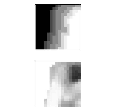
5.4.2.1 Grey Shape Coding
Binary shape coding (described in Section 5.4.1.1) has certain drawbacks in the representation of video scenes made up of multiple objects. Objects or regions in a ‘natural’ video scene may be translucent (partially transparent) but binary shape coding only supports completely transparent (‘invisible’) or completely opaque regions. It is often difficult or impossible to segment video objects neatly (since object boundaries may not exactly correspond with pixel positions), especially when segmentation is carried out automatically or semi-automatically.
• |
MPEG-4 VISUAL |
134 |
Figure 5.42 Grey-scale alpha mask for boundary MB
Figure 5.43 Boundary MB with grey-scale transparency
For example, the edge of the VOP shown in Figure 5.30 is not entirely ‘clean’ and this may lead to unwanted artefacts around the VOP edge when it is rendered with other VOs.
Grey shape coding gives more flexible control of object transparency. A grey-scale alpha plane is coded for each macroblock, in which each pixel position has a mask value between 0 and 255, where 0 indicates that the pixel position is fully transparent, 255 indicates that it is fully opaque and other values specify an intermediate level of transparency. An example of a grey-scale mask for a boundary MB is shown in Figure 5.42. The transparency ranges from fully transparent (black mask pixels) to opaque (white mask pixels). The rendered MB is shown in Figure 5.43 and the edge of the object now ‘fades out’ (compare this figure with Figure 5.32). Figure 5.44 is a scene constructed of a background VO (rectangular) and two foreground VOs. The foreground VOs are identical except for their transparency, the left-hand VO uses a binary alpha mask and the right-hand VO has a grey alpha mask which helps the right-hand VO to blend more smoothly with the background. Other uses of grey shape coding include representing translucent objects, or deliberately altering objects to make them semi-transparent (e.g. the synthetic scene in Figure 5.45).
CODING ARBITRARY-SHAPED REGIONS |
• |
|
135 |
|
|
Figure 5.44 Video scene with binary-alpha object (left) and grey-alpha object (right)
Figure 5.45 Video scene with semi-transparent object
Grey scale alpha masks are coded using two components, a binary support mask that indicates which pixels are fully transparent (external to the VO) and which pixels are semior fully-opaque (internal to the VO), and a grey scale alpha plane. Figure 5.33 is the binary support mask for the grey-scale alpha mask of Figure 5.42. The binary support mask is coded in the same way as a BAB (see Section 5.4.1.1). The grey scale alpha plane (indicating the level of transparency of the internal pixels) is coded separately in the same way as object texture (i.e. each 8 × 8 block within the alpha plane is transformed using the DCT, quantised,
• |
MPEG-4 VISUAL |
136 |
Figure 5.46 Sequence of frames
reordered, run-level and entropy coded). The decoder reconstructs the grey scale alpha plane (which may not be identical to the original alpha plane due to quantisation distortion) and the binary support mask. If the binary support mask indicates that a pixel is outside the VO, the corresponding grey scale alpha plane value is set to zero. In this way, the object boundary is accurately preserved (since the binary support mask is losslessly encoded) whilst the decoded grey scale alpha plane (and hence the transparency information) may not be identical to the original.
The increased flexibility provided by grey scale alpha shape coding is achieved at a cost of reduced compression efficiency. Binary shape coding requires the transmission of BABs for each boundary MB and in addition, grey scale shape coding requires the transmission of grey scale alpha plane data for every MB that is semi-transparent.
5.4.2.2 Static Sprite Coding
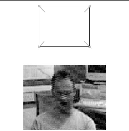
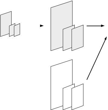
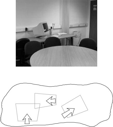
Three frames from a video sequence are shown in Figure 5.46. Clearly, the background does not change during the sequence (the camera position is fixed). The background (Figure 5.47) may be coded as a static sprite. A static sprite is treated as a texture image that may move or warp in certain limited ways, in order to compensate for camera changes such as pan, tilt, rotation and zooming. In a typical scenario, a sprite may be much larger than the visible area of the scene. As the camera ‘viewpoint’ changes, the encoder transmits parameters indicating how the sprite should be moved and warped to recreate the appropriate visible area in the decoded scene. Figure 5.48 shows a background sprite (the large region) and the area viewed by the camera at three different points in time during a video sequence. As the sequence progresses, the sprite is moved, rotated and warped so that the visible area changes appropriately. A sprite may have arbitrary shape (Figure 5.48) or may be rectangular.
The use of static sprite coding is indicated by setting sprite enable to ‘Static’ in a VOL header, after which static sprite coding is used throughout the VOP. The first VOP in a static sprite VOL is an I-VOP and this is followed by a series of S-VOPs (Static Sprite VOPs). Note that a Static Sprite S-VOP is coded differently from a Global Motion Compensation S(GMC)- VOP (described in Section 5.3.3).There are two methods of transmitting and manipulating sprites, a ‘basic’ sprite (sent in its entirety at the start of a sequence) and a ‘low-latency’ sprite (updated piece by piece during the sequence).
CODING ARBITRARY-SHAPED REGIONS |
• |
|
137 |
|
|
Figure 5.47 Background sprite
background sprite
2
3
1
Figure 5.48 Background sprite and three different camera viewpoints
Basic Sprite
The first VOP (I-VOP) contains the entire sprite, encoded in the same way as a ‘normal’ I-VOP. The sprite may be larger than the visible display size (to accommodate camera movements during the sequence). At the decoder, the sprite is placed in a Sprite Buffer and is not immediately displayed. All further VOPs in the VOL are S-VOPs. An S-VOP contains up to four warping parameters that are used to move and (optionally) warp the contents of the Sprite Buffer in order to produce the desired background display. The number of warping parameters per S-VOP (up to four) is chosen in the VOL header and determines the flexibility of the Sprite Buffer transformation. A single parameter per S-VOP enables linear translation (i.e. a single motion vector for the entire sprite), two or three parameters enable affine

• |
MPEG-4 VISUAL |
138 |
transformation of the sprite (e.g. rotation, shear) and four parameters enable a perspective transform.
Low-latency sprite
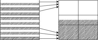
Transmitting an entire sprite in Basic Sprite mode at the start of a VOL may introduce significant latency because the sprite may be much larger than an individual displayed VOP. The Low-Latency Sprite mode enables an encoder to send initially a minimal size and/or lowquality version of the sprite and then update it during transmission of the VOL. The first I-VOP contains part or all of the sprite (optionally encoded at a reduced quality to save bandwidth) together with the height and width of the entire sprite.
Each subsequent S-VOP may contain warping parameters (as in the Basic Sprite mode) and one or more sprite ‘pieces’. A sprite ‘piece’ covers a rectangular area of the sprite and contains macroblock data that (a) constructs part of the sprite that has not previously been decoded (‘static-sprite-object’ piece) or (b) improves the quality of part of the sprite that has been previously decoded (‘static-sprite-update’ piece). Macroblocks in a ‘static-sprite- object’ piece are encoded as intra macroblocks (including shape information if the sprite is not rectangular). Macroblocks in a ‘static-sprite-update’ piece are encoded as inter macroblocks using forward prediction from the previous contents of the sprite buffer (but without motion vectors or shape information).
Example
The sprite shown in Figure 5.47 is to be transmitted in low-latency mode. The initial I-VOP contains a low-quality version of part of the sprite and Figure 5.49 shows the contents of the sprite buffer after decoding the I-VOP. An S-VOP contains a new piece of the sprite, encoded in high-quality mode (Figure 5.50) and this extends the contents of the sprite buffer (Figure 5.51). A further S-VOP contains a residual piece (Figure 5.52) that improves the quality of the top-left part of the current sprite buffer. After adding the decoded residual, the sprite buffer contents are as shown Figure 5.53. Finally, four warping points are transmitted in a further S-VOP to produce a change of rotation and perspective (Figure 5.54).
5.4.3 The Advanced Coding Efficiency Profile
The ACE profile is a superset of the Core profile that supports coding of grey-alpha video objects with high compression efficiency. In addition to Simple and Core objects, it includes the ACE object which adds the following tools:
quarter-pel motion compensation (Section 5.3.3);
GMC (Section 5.3.3);
interlace (Section 5.3.3);
grey shape coding (Section 5.4.2);
shape-adaptive DCT.
The Shape-Adaptive DCT (SA-DCT) is based on pre-defined sets of one-dimensional DCT basis functions and allows an arbitrary region of a block to be efficiently transformed and compressed. The SA-DCT is only applicable to 8 × 8 blocks within a boundary BAB that
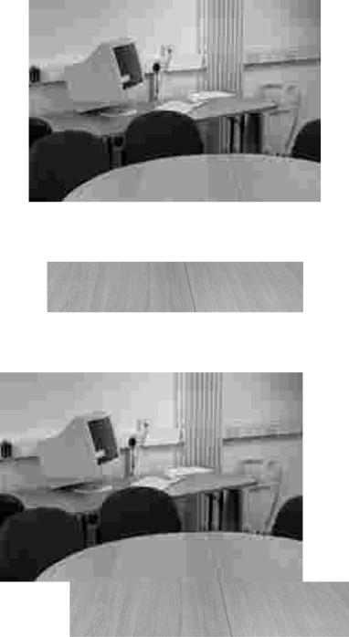
CODING ARBITRARY-SHAPED REGIONS |
• |
|
139 |
|
|
Figure 5.49 Low-latency sprite: decoded I-VOP
Figure 5.50 Low-latency sprite: static-sprite-object piece
Figure 5.51 Low-latency sprite: buffer contents (1)
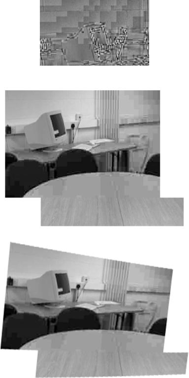
Figure 5.52 Low-latency sprite: static-sprite-update piece
Figure 5.53 Low-latency sprite: buffer contents (2)
Figure 5.54 Low-latency sprite: buffer contents (3)
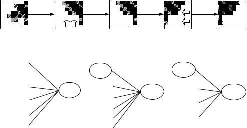
CODING ARBITRARY-SHAPED REGIONS |
• |
|
141 |
|
|
Residual X |
Residual X |
Intermediate Y |
Intermediate Y |
Shift |
1-D column |
Shift |
vertically |
DCT |
horizontally |
Figure 5.55 Shape-adaptive DCT
Coefficients Z
1-D row |
DCT |
I-VOP |
|
|
|
|
|
P-VOP |
|
|
|
|
|
4MV |
|
|
|
|
|
UMV |
|
|
|
Core |
|
Intra Pred |
|
Simple |
|
|
|
|
|
|
|
||
|
|
|
|
|
|
Video packets |
|
|
|
Temporal |
|
Data Partitioning |
Simple |
FGS |
Fine Granular |
Scalability |
|
RVLCs |
|
Core Scalable |
|||
Scalable |
|
(rectangular) |
|||
|
|
Scalability |
|||
|
|
FGS Temporal |
|
|
|
B-VOP |
|
Scalability |
|
Spatial Scalability |
|
|
|
|
|
(rectangular) |
|
Temporal |
|
Interlace |
|
|
|
Scalability |
|
|
|
Object-based |
|
(rectangular) |
|
B-VOP |
|
spatial scalability |
|
|
|
|
|
|
|
|
|
|
|
|
|
Spatial Scalability |
|
Alternate Quant |
|
|
|
(rectangular) |
|
|
|
|
|
Figure 5.56 Tools and objects for scalable coding
contain one or more transparent pixels. The Forward SA-DCT consists of the following steps (Figure 5.55):
1.Shift opaque residual values X to the top of the 8 × 8 block.
2.Apply a 1D DCT to each column (the number of points in the transform matches the number of opaque values in each column).
3.Shift the resulting intermediate coefficients Y to the left of the block.
4.Apply a 1D DCT to each row (matched to the number of values in each row).
The final coefficients (Z) are quantised, zigzag scanned and encoded. The decoder reverses the process (making use of the shape information decoded from the BAB) to reconstruct the 8 × 8 block of samples. The SA-DCT is more complex than the normal 8 × 8 DCT but can improve coding efficiency for boundary MBs.
5.4.4 The N-bit Profile
The N-bit profile contains Simple and Core objects plus the N-bit tool. This supports coding of luminance and chrominance data containing between four and twelve bits per sample (instead of the usual restriction to eight bits per sample). Possible applications of the N-bit profile include video coding for displays with low colour depth (where the limited display capability means that less than eight bits are required to represent each sample) or for high-quality display applications (where the display has a colour depth of more than eight bits per sample and high coded fidelity is desired).