6.6 THE EXTENDED PROFILE

The Extended Profile (known as the X Profile in earlier versions of the draft H.264 standard) may be particularly useful for applications such as video streaming. It includes all of the features of the Baseline Profile (i.e. it is a superset of the Baseline Profile, unlike Main Profile), together with B-slices (Section 6.5.1), Weighted Prediction (Section 6.5.2) and additional features to support efficient streaming over networks such as the Internet. SP and SI slices facilitate switching between different coded streams and ‘VCR-like’ functionality and Data Partitioned slices can provide improved performance in error-prone transmission environments.

6.6.1 SP and SI slices

SP and SI slices are specially-coded slices that enable (among other things) efficient switching between video streams and efficient random access for video decoders [10]. A common requirement in a streaming application is for a video decoder to switch between one of several encoded streams. For example, the same video material is coded at multiple bitrates for transmission across the Internet and a decoder attempts to decode the highest-bitrate stream it can receive but may require switching automatically to a lower-bitrate stream if the data throughput drops.

Example

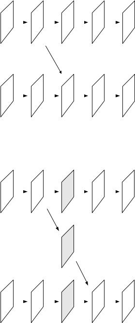
A decoder is decoding Stream A and wants to switch to decoding Stream B (Figure 6.48). For simplicity, assume that each frame is encoded as a single slice and predicted from one reference (the previous decoded frame). After decoding P-slices A0 and A1 , the decoder wants to switch to Stream B and decode B2 , B3 and so on. If all the slices in Stream B are coded as P-slices, then the decoder will not have the correct decoded reference frame(s) required to reconstruct B2 (since B2 is predicted from the decoded picture B1 which does not exist in stream A). One solution is to code frame B2 as an I-slice. Because it is coded without prediction from any other frame, it can be decoded independently of preceding frames in stream B and the decoder can therefore switch between stream A and stream B as shown in Figure 6.49. Switching can be accommodated by inserting an I-slice at regular intervals in the coded sequence to create ‘switching points’. However, an I-slice is likely to contain much more coded data than a P-slice and the result is an undesirable peak in the coded bitrate at each switching point.

SP-slices are designed to support switching between similar coded sequences (for example, the same source sequence encoded at various bitrates) without the increased bitrate penalty of I-slices (Figure 6.49). At the switching point (frame 2 in each sequence), there are three SP-slices, each coded using motion compensated prediction (making them more efficient than I-slices). SP-slice A2 can be decoded using reference picture A1 and SP-slice B2 can be decoded using reference picture B1. The key to the switching process is SP-slice AB2 (known as a switching SP-slice), created in such a way that it can be decoded using motioncompensated reference picture A1, to produce decoded frame B2 (i.e. the decoder output frame B2 is identical whether decoding B1 followed by B2 or A1 followed by AB2). An extra SP-slice is required at each switching point (and in fact another SP-slice, BA2, would be required to switch in the other direction) but this is likely to be more efficient than encoding frames A2

and B2 as I-slices. Table 6.18 lists the steps involved when a decoder switches from stream A to stream B.

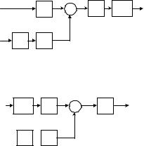
Figure 6.50 shows a simplified diagram of the encoding process for SP-slice A2, produced by subtracting a motion-compensated version of A1 (decoded frame A1) from frame A2 and then coding the residual. Unlike a ‘normal’ P-slice, the subtraction occurs in the transform domain (after the block transform). SP-slice B2 is encoded in the same way (Figure 6.51). A decoder that has previously decoded frame A1 can decode SP-slice A2 as shown in Figure 6.52. Note that these diagrams are simplified; in practice further quantisation and rescaling steps are required to avoid mismatch between encoder and decoder and a more detailed treatment of the process can be found in [11].