

142 |
|
|
|
|
|
|
|
|
|
|
|
|
|
|
MPEG-4 VISUAL |
|
|
|
|
|
|
|
|
|
|
|
|
|
|
|
|
|
|
• video |
|
|
|
|
|
|
|
|
|
|
|
|
|
|
basic-quality |
|
|
|
|
|
|
base layer |
|
|
|
|
|
|
decoder A |
|
|||
|
|
encoder |
|
|
enhancement |
|
|
|
|
|
|
|
sequence |
|||
|
|
|
|
|
|
|
||||||||||
|
|
|
||||||||||||||
|
|
|
|
|
|
|||||||||||
|
sequence |
|
|
|
layer 1 |
|
|
|
|
|
|
|||||
|
|
|
|
|
|
... |
|
|
|
|
|
|
|
|
|
|
|
|
|
|
|
|
|
enhancement |
|
|
|
|
|
|
|
high-quality |
|
|
|
|
|
|
|
|
|
|
|
|
decoder B |
|
||||
|
|
|
|
|
|
|
|
|
|
|||||||
|
|
|
|
|
|
|
layer N |
|
|
|
sequence |
|||||
|
|
|
|
|
|
|
|
|
|
|
|
|
|
|
|
|
|
|
|
|
|
|
|
|
|
|
|
|
|
|
|
|
|
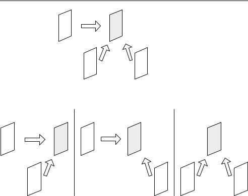
Figure 5.57 Scalable coding: general concept
5.5 SCALABLE VIDEO CODING
Scalable encoding of video data enables a decoder to decode selectively only part of the coded bitstream. The coded stream is arranged in a number of layers, including a ‘base’ layer and one or more ‘enhancement’ layers (Figure 5.57). In this figure, decoder A receives only the base layer and can decode a ‘basic’ quality version of the video scene, whereas decoder B receives all layers and decodes a high quality version of the scene. This has a number of applications, for example, a low-complexity decoder may only be capable of decoding the base layer; a low-rate bitstream may be extracted for transmission over a network segment with limited capacity; and an error-sensitive base layer may be transmitted with higher priority than enhancement layers.
MPEG-4 Visual supports a number of scalable coding modes. Spatial scalability enables a (rectangular) VOP to be coded at a hierarchy of spatial resolutions. Decoding the base layer produces a low-resolution version of the VOP and decoding successive enhancement layers produces a progressively higher-resolution image. Temporal scalability provides a low frame-rate base layer and enhancement layer(s) that build up to a higher frame rate. The standard also supports quality scalability, in which the enhancement layers improve the visual quality of the VOP and complexity scalability, in which the successive layers are progressively more complex to decode. Fine Grain Scalability (FGS) enables the quality of the sequence to be increased in small steps. An application for FGS is streaming video across a network connection, in which it may be useful to scale the coded video stream to match the available bit rate as closely as possible.
5.5.1 Spatial Scalability
The base layer contains a reduced-resolution version of each coded frame. Decoding the base layer alone produces a low-resolution output sequence and decoding the base layer with enhancement layer(s) produces a higher-resolution output. The following steps are required to encode a video sequence into two spatial layers:
1.Subsample each input video frame (Figure 5.58) (or video object) horizontally and vertically (Figure 5.59).
2.Encode the reduced-resolution frame to form the base layer.
3.Decode the base layer and up-sample to the original resolution to form a prediction frame (Figure 5.60).
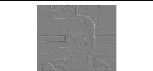
4.Subtract the full-resolution frame from this prediction frame (Figure 5.61).
5.Encode the difference (residual) to form the enhancement layer.
SCALABLE VIDEO CODING |
• |
|
143 |
|
|
Figure 5.58 Original video frame
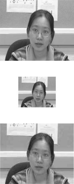
Figure 5.59 Sub-sampled frame to be encoded as base layer
Figure 5.60 Base layer frame (decoded and upsampled)
• |
MPEG-4 VISUAL |
144 |
Figure 5.61 Residual to be encoded as enhancement layer
A single-layer decoder decodes only the base layer to produce a reduced-resolution output sequence. A two-layer decoder can reconstruct a full-resolution sequence as follows:
1.Decode the base layer and up-sample to the original resolution.
2.Decode the enhancement layer.
3.Add the decoded residual from the enhancement layer to the decoded base layer to form the output frame.
An I-VOP in an enhancement layer is encoded without any spatial prediction, i.e. as a complete frame or object at the enhancement resolution. In an enhancement layer P-VOP, the decoded, up-sampled base layer VOP (at the same position in time) is used as a prediction without any motion compensation. The difference between this prediction and the input frame is encoded using the texture coding tools, i.e. no motion vectors are transmitted for an enhancement P-VOP. An enhancement layer B-VOP is predicted from two directions. The backward prediction is formed by the decoded, up-sampled base layer VOP (at the same position in time), without any motion compensation (and hence without any MVs). The forward prediction is formed by the previous VOP in the enhancement layer (even if this is itself a B-VOP), with motion-compensated prediction (and hence MVs).
If the VOP has arbitrary (binary) shape, a base layer and enhancement layer BAB is required for each MB. The base layer BAB is encoded as usual, based on the shape and size of the base layer object. A BAB in a P-VOP enhancement layer is coded using prediction from an up-sampled version of the base layer BAB. A BAB in a B-VOP enhancement layer may be coded in the same way, or using forward prediction from the previous enhancement VOP (as described in Section 5.4.1.1).
5.5.2 Temporal Scalability
The base layer of a temporal scalable sequence is encoded at a low video frame rate and a temporal enhancement layer consists of I-, P- and/or B-VOPs that can be decoded together with the base layer to provide an increased video frame rate. Enhancement layer VOPs are predicted using motion-compensated prediction according to the following rules.
SCALABLE VIDEO CODING |
|
|
|
|
145 |
0 |
(i) |
2 |
|
enhancement |
• |
|
|
|
|
layer VOPs |
|
|
(ii) |
(iii) |
|
base layer |
|
|
1 |
|
3 |
VOPs |
|
Figure 5.62 Temporal enhancement P-VOP prediction options
0 |
2 |
0 |
2 |
2 |
1 |
3 |
1 |
3 |
(i) |
(ii) |
(iii) |
|
Figure 5.63 Temporal enhancement B-VOP prediction options
An enhancement I-VOP is encoded without any prediction. An enhancement P-VOP is predicted from (i) the previous enhancement VOP, (ii) the previous base layer VOP or (iii) the next base layer VOP (Figure 5.62). An enhancement B-VOP is predicted from (i) the previous enhancement and previous base layer VOPs, (ii) the previous enhancement and next base layer VOPs or (iii) the previous and next base layer VOPs (Figure 5.63).
5.5.3 Fine Granular Scalability
Fine Granular Scalability (FGS) [5] is a method of encoding a sequence as a base layer and enhancement layer. The enhancement layer can be truncated during or after encoding (reducing the bitrate and the decoded quality) to give highly flexible control over the transmitted bitrate. FGS may be useful for video streaming applications, in which the available transmission bandwidth may not be known in advance. In a typical scenario, a sequence is coded as a base layer and a high-quality enhancement layer. Upon receiving a request to send the sequence at a particular bitrate, the streaming server transmits the base layer and a truncated version of the enhancement layer. The amount of truncation is chosen to match the available transmission bitrate, hence maximising the quality of the decoded sequence without the need to re-encode the video clip.
146 |
|
|
|
|
|
|
|
|
|
MPEG-4 VISUAL |
|
|
|
|
|
|
|
|
|
|
|
|
|
•Texture |
|
|
|
|
|
|
|
|
|
Base |
|
|
FDCT |
|
|
Quant |
|
|
Encode |
|
|||
|
|
|
|
|
coefficients |
|
layer |
||||
|
|
Rescale |
|
|
- |
Encode |
Enhancement |
|
|
||
|
|
each |
|
+ |
|
layer |
|
|
bitplane |
||
|
|
|
Figure 5.64 FGS encoder block diagram (simplified)
13 |
-11 |
0 |
0 |
... |
0 |
17 |
0 |
... |
|
0 |
-3 ... |
|
|
|
0 |
... |
|
|
|
... |
|
|
|
|
Figure 5.65 Block of residual coefficients (top-left corner)
Encoding
Figure 5.64 shows a simplified block diagram of an FGS encoder (motion compensation is not shown). In the Base Layer, the texture (after motion compensation) is transformed with the forward DCT, quantised and encoded. The quantised coefficients are re-scaled (‘inverse quantised’) and these re-scaled coefficients are subtracted from the unquantised DCT coefficients to give a set of difference coefficients. The difference coefficients for each block are encoded as a series of bitplanes. First, the residual coefficients are reordered using a zigzag scan. The highest-order bits of each coefficient (zeros or ones) are encoded first (the MS bitplane) followed by the next highest-order bits and so on until the LS bits have been encoded.
Example
A block of residual coefficients is shown in Figure 5.65 (coefficients not shown are zero). The coefficients are reordered in a zigzag scan to produce the following list:
+13, −11, 0, 0, +17, 0, 0, 0, −3, 0, 0 . . . .
The bitplanes corresponding to the magnitude of each residual coefficient are shown in Table 5.6. In this case, the highest plane containing nonzero bits is plane 4 (because the highest magnitude is 17).

SCALABLE VIDEO CODING |
|
|
|
|
|
|
|
|
|
147 |
|
|||
|
|
|
|
|
|
|
|
|||||||
|
|
Table |
5.6 |
Residual coefficient bitplanes (magnitude) |
|
• |
||||||||
|
|
|
|
|
|
|
|
|
|
|
|
|||
|
Value |
|
+13 |
−11 |
0 |
0 |
+17 |
0 |
0 |
0 |
−3 |
0 . . . |
||
|
Plane 4 (MSB) |
0 |
0 |
0 |
0 |
1 |
0 |
0 |
0 |
0 |
0 . . . |
|
|
|
|
Plane 3 |
|
1 |
1 |
0 |
0 |
0 |
0 |
0 |
0 |
0 |
0 . . . |
|
|
|
Plane 2 |
|
1 |
1 |
0 |
0 |
0 |
0 |
0 |
0 |
0 |
0 . . . |
|
|
|
Plane 1 |
|
0 |
0 |
0 |
0 |
0 |
0 |
0 |
0 |
1 |
0 . . . |
|
|
|
Plane 0 (LSB) |
1 |
1 |
0 |
0 |
1 |
0 |
0 |
0 |
1 |
0 . . . |
|
|
|
|
|
|
|
|
|
|
|
|
|
|
|
|||
|
|
|
|
Table 5.7 |
Encoded values |
|
|
|
|
|
|
|||
|
|
|
|
|
|
|
|
|
|
|
|
|
||
|
|
|
|
Plane |
|
Encoded values |
|
|
|
|
|
|
||
4(4, EOP) (+)
3 (0) (+) (0, EOP) (−)
2(0, EOP)
1(1) (6, EOP) (−)
0(0) (0) (2) (3, EOP)
Each bitplane contains a series of zeros and ones. The ones are encoded as (run, EOP) where ‘EOP’ indicates ‘end of bitplane’ and each (run, EOP) pair is transmitted as a variable-length code. Whenever the MS bit of a coefficient is encoded, it is immediately followed in the bitstream by a sign bit. Table 5.7 lists the encoded values for each bitplane. Bitplane 4 contains four zeros, followed by a 1. This is the last nonzero bit and so is encoded as (4, EOP). This also the MS bit of the coefficient ‘+17’ and so the sign of this coefficient is encoded.
This example illustrates the processing of one block. The encoding procedure for a complete frame is as follows:
1.Find the highest bit position of any difference coefficient in the frame (the MSB).
2.Encode each bitplane as described above, starting with the plane containing the MSB.
Each complete encoded bitplane is preceded by a start code, making it straightforward to truncate the bitstream by sending only a limited number of encoded bitplanes.
Decoding
The decoder decodes the base layer and enhancement layer (which may be truncated). The difference coefficients are reconstructed from the decoded bitplanes, added to the base layer coefficients and inverse transformed to produce the decoded enhancement sequence (Figure 5.66).
If the enhancement layer has been truncated, then the accuracy of the difference coefficients is reduced. For example, assume that the enhancement layer described in the above example is truncated after bitplane 3. The MS bits (and the sign) of the first three nonzero coefficients are decoded (Table 5.8); if the remaining (undecoded) bitplanes are filled with

• |
|
|
|
|
|
|
|
|
|
|
|
|
|
|
|
|
|
|
|
|
MPEG-4 VISUAL |
|||
148 |
|
|
|
|
|
|
|
|
|
|
|
|
|
|
|
|
|
|
|
|
||||
|
|
|
|
Table 5.8 Decoded values (truncated after plane 3) |
|
|
|
|||||||||||||||||
|
|
|
|
|
|
|
|
|
|
|
|
|
|
|
|
|
|
|
|
|
|
|
|
|
|
|
Plane 4 (MSB) |
0 |
|
0 |
0 |
0 |
|
|
1 |
|
0 |
|
0 |
0 |
0 |
0 . . . |
|
|
|||||
|
|
Plane 3 |
1 |
1 |
0 |
0 |
|
|
0 |
0 |
|
0 |
0 |
0 |
0 . . . |
|
|
|||||||
|
|
Plane 2 |
0 |
0 |
0 |
0 |
|
|
0 |
0 |
|
0 |
0 |
0 |
0 . . . |
|
|
|||||||
|
|
Plane 1 |
0 |
0 |
0 |
0 |
|
|
0 |
0 |
|
0 |
0 |
0 |
0 . . . |
|
|
|||||||
|
|
Plane 0 (LSB) |
0 |
0 |
0 |
0 |
|
|
0 |
0 |
|
0 |
0 |
0 |
0 . . . |
|
|
|||||||
|
|
Decoded value |
+8 |
−8 |
0 |
0 |
|
|
+16 |
0 |
|
0 |
0 |
0 |
0 . . . |
|
|
|||||||
|
|
|
|
|
|
|
|
|
|
|
|
|
|
|
|
|
|
|
|
|
|
|
|
|
|
Base |
|
|
Decode |
|
|
|
|
Rescale |
|
|
|
|
|
|
|
|
IDCT |
|
|
|
|
Texture |
|
|
layer |
|
|
coefficients |
|
|
|
|
|
|
|
|
|
|
|
|
|
|
|
|
|
|
(base layer) |
|
|
Enhancement |
|
|
|
|
|
|
|
|
|
|
|
|
|
+ |
|
|
|
|
|
|
|
Texture |
|
|
|
|
|
|
|
|
|
|
+ |
|
|
|
|
|
|
|
|
|
||||||
|
|
|
Decode |
|
|
|
|
|
|
|
|
|
|
|
|
|
|
|||||||
|
layer (may be |
|
|
|
|
|
|
|
|
|
|
|
|
|
|
|
|
|
|
|||||
|
|
|
|
|
|
|
|
|
|
|
|
|
|
|
|
|
IDCT |
|
|
|
|
(enhancement |
||
|
truncated) |
|
|
bitplanes |
|
|
|
|
|
|
|
|
|
|
|
|
|
|
|
|
|
|
layer) |
|
|
|
|
|
|
|
|
|
|
|
|
|
|
|
|
|
|
|
|
|
|
|
|
||
Figure 5.66 FGS decoder block diagram (simplified)
zeros then the list of output values becomes:
+8, −8, 0, 0, +16, 0 . . . .
Optional enhancements to FGS coding include selective enhancement (in which bit planes of selected MBs are bit-shifted up prior to encoding, in order to give them a higher priority and a higher probability of being included in a truncated bitstream) and frequency weighting (in which visually-significant low frequency DCT coefficients are shifted up prior to encoding, again in order to give them higher priority in a truncated bitstream).
5.5.4 The Simple Scalable Profile
The Simple Scalable profile supports Simple and Simple Scalable objects. The Simple Scalable object contains the following tools:
I-VOP, P-VOP, 4MV, unrestricted MV and Intra Prediction;
Video packets, Data Partitioning and Reversible VLCs;
B-VOP;
Rectangular Temporal Scalability (1 enhancement layer) (Section 5.5.2);
Rectangular Spatial Scalability (1 enhancement layer) (Section 5.5.1).
The last two tools support scalable coding of rectangular VOs.
5.5.5 The Core Scalable Profile
The Core Scalable profile includes Simple, Simple Scalable and Core objects, plus the Core Scalable object which features the following tools, in each case with up to two enhancement layers per object: