

ENTROPY CODER |
• |
|
61 |
|
|
3.5 ENTROPY CODER
The entropy encoder converts a series of symbols representing elements of the video sequence into a compressed bitstream suitable for transmission or storage. Input symbols may include quantised transform coefficients (run-level or zerotree encoded as described in Section 3.4.4), motion vectors (an x and y displacement vector for each motion-compensated block, with integer or sub-pixel resolution), markers (codes that indicate a resynchronisation point in the sequence), headers (macroblock headers, picture headers, sequence headers, etc.) and supplementary information (‘side’ information that is not essential for correct decoding). In this section we discuss methods of predictive pre-coding (to exploit correlation in local regions of the coded frame) followed by two widely-used entropy coding techniques, ‘modified Huffman’ variable length codes and arithmetic coding.
3.5.1 Predictive Coding
Certain symbols are highly correlated in local regions of the picture. For example, the average or DC value of neighbouring intra-coded blocks of pixels may be very similar; neighbouring motion vectors may have similar x and y displacements and so on. Coding efficiency may be improved by predicting elements of the current block or macroblock from previously-encoded data and encoding the difference between the prediction and the actual value.
The motion vector for a block or macroblock indicates the offset to a prediction reference in a previously-encoded frame. Vectors for neighbouring blocks or macroblocks are often correlated because object motion may extend across large regions of a frame. This is especially true for small block sizes (e.g. 4 × 4 block vectors, see Figure 3.22) and/or large moving objects. Compression of the motion vector field may be improved by predicting each motion vector from previously-encoded vectors. A simple prediction for the vector of the current macroblock X is the horizontally adjacent macroblock A (Figure 3.44), alternatively three or more previously-coded vectors may be used to predict the vector at macroblock X (e.g. A, B and C in Figure 3.44). The difference between the predicted and actual motion vector (Motion Vector Difference or MVD) is encoded and transmitted.
The quantisation parameter or quantiser step size controls the tradeoff between compression efficiency and image quality. In a real-time video CODEC it may be necessary to modify the quantisation within an encoded frame (for example to alter the compression ratio in order to match the coded bit rate to a transmission channel rate). It is usually
B C
AX
Figure 3.44 Motion vector prediction candidates

• |
VIDEO CODING CONCEPTS |
62 |
sufficient (and desirable) to change the parameter only by a small amount between successive coded macroblocks. The modified quantisation parameter must be signalled to the decoder and instead of sending a new quantisation parameter value, it may be preferable to send a delta or difference value (e.g. ±1 or ±2) indicating the change required. Fewer bits are required to encode a small delta value than to encode a completely new quantisation parameter.
3.5.2 Variable-length Coding
A variable-length encoder maps input symbols to a series of codewords (variable length codes or VLCs). Each symbol maps to a codeword and codewords may have varying length but must each contain an integral number of bits. Frequently-occurring symbols are represented with short VLCs whilst less common symbols are represented with long VLCs. Over a sufficiently large number of encoded symbols this leads to compression of the data.
3.5.2.1 Huffman Coding
Huffman coding assigns a VLC to each symbol based on the probability of occurrence of different symbols. According to the original scheme proposed by Huffman in 1952 [7], it is necessary to calculate the probability of occurrence of each symbol and to construct a set of variable length codewords. This process will be illustrated by two examples.
Example 1: Huffman coding, sequence 1 motion vectors
The motion vector difference data (MVD) for a video sequence (‘sequence 1’) is required to be encoded. Table 3.2 lists the probabilities of the most commonly-occurring motion vectors in the encoded sequence and their information content, log2 (1/ p). To achieve optimum compression, each value should be represented with exactly log2 (1/ p) bits. ‘0’ is the most common value and the probability drops for larger motion vectors (this distribution is representative of a sequence containing moderate motion).
Table 3.2 Probability of occurrence of motion vectors in sequence 1
Vector |
Probability p |
log2(1/ p) |
|
|
|
−2 |
0.1 |
3.32 |
−1 |
0.2 |
2.32 |
0 |
0.4 |
1.32 |
1 |
0.2 |
2.32 |
2 |
0.1 |
3.32 |
|
|
|
ENTROPY CODER |
|
|
63 |
|
0 |
-2 p = 0.1 |
• |
|
A p = 0.2 |
|
|
0 |
1 |
2 p = 0.1 |
|
|
|
|
|
C |
|
|
|
0 |
|
-1 p = 0.2 |
|
1 0
Dp =1.0
|
|
|
B p = 0.4 |
||
1 |
|
|
1 |
|
|
|
0 |
p = 0.4 |
1 |
p = 0.2 |
|
|
|
||||
|
|
|
|
|
|
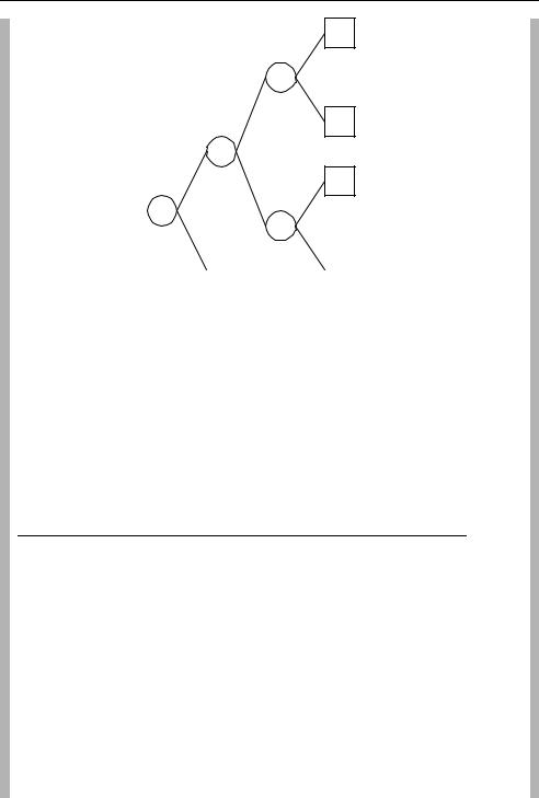
Figure 3.45 Generating the Huffman code tree: sequence 1 motion vectors
1. Generating the Huffman Code Tree
To generate a Huffman code table for this set of data, the following iterative procedure is carried out:
1.Order the list of data in increasing order of probability.
2.Combine the two lowest-probability data items into a ‘node’ and assign the joint probability of the data items to this node.
3.Re-order the remaining data items and node(s) in increasing order of probability and repeat step 2.
The procedure is repeated until there is a single ‘root’ node that contains all other nodes and data items listed ‘beneath’ it. This procedure is illustrated in Figure 3.45.
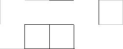
Original list: |
The data items are shown as square boxes. Vectors (−2) and (+2) have the |
|
lowest probability and these are the first candidates for merging to form |
|
node ‘A’. |
Stage 1: |
The newly-created node ‘A’ (shown as a circle) has a probability of 0.2 |
|
(from the combined probabilities of (−2) and (2)). There are now three items |
|
with probability 0.2. Choose vectors (−1) and (1) and merge to form |
|
node ‘B’. |
Stage 2: |
A now has the lowest probability (0.2) followed by B and the vector 0; |
|
choose A and B as the next candidates for merging (to form ‘C’). |
Stage 3: |
Node C and vector (0) are merged to form ‘D’. |
Final tree: |
The data items have all been incorporated into a binary ‘tree’ containing five |
|
data values and four nodes. Each data item is a ‘leaf’ of the tree. |
|
|
2. Encoding
Each ‘leaf’ of the binary tree is mapped to a variable-length code. To find this code, the tree is traversed from the root node (D in this case) to the leaf (data item). For every branch, a 0 or 1

64 |
|
|
|
|
VIDEO CODING CONCEPTS |
||
|
|
|
|
|
|
||
• |
Table 3.3 |
Huffman codes for sequence 1 |
|||||
|
motion vectors |
|
|
||||
|
|
Vector |
Code |
Bits (actual) |
Bits (ideal) |
||
|
|
|
|
|
|
|
|
|
|
0 |
|
1 |
1 |
1.32 |
|
|
|
1 |
011 |
3 |
2.32 |
|
|
|
|
−1 |
010 |
3 |
2.32 |
|
|
|
|
2 |
001 |
3 |
3.32 |
|
|
|
|
−2 |
000 |
3 |
3.32 |
|
|
Table 3.4 Probability of occurrence of motion vectors in sequence 2
Vector |
Probability |
log2 (1/ p) |
−2 |
0.02 |
5.64 |
−1 |
0.07 |
3.84 |
0 |
0.8 |
0.32 |
1 |
0.08 |
3.64 |
2 |
0.03 |
5.06 |
|
|
|
is appended to the code, 0 for an upper branch, 1 for a lower branch (shown in the final tree of Figure 3.45), giving the following set of codes (Table 3.3).
Encoding is achieved by transmitting the appropriate code for each data item. Note that once the tree has been generated, the codes may be stored in a look-up table.
High probability data items are assigned short codes (e.g. 1 bit for the most common vector ‘0’). However, the vectors (−2, 2, −1, 1) are each assigned three-bit codes (despite the fact that –1 and 1 have higher probabilities than –2 and 2). The lengths of the Huffman codes (each an integral number of bits) do not match the ideal lengths given by log2 (1/ p). No code contains any other code as a prefix which means that, reading from the left-hand bit, each code is uniquely decodable.
For example, the series of vectors (1, 0, −2) would be transmitted as the binary sequence 0111000.
3. Decoding
In order to decode the data, the decoder must have a local copy of the Huffman code tree (or look-up table). This may be achieved by transmitting the look-up table itself or by sending the list of data and probabilities prior to sending the coded data. Each uniquely-decodeable code is converted back to the original data, for example:
011 is decoded as (1)
1 is decoded as (0)
000 is decoded as (−2).
Example 2: Huffman coding, sequence 2 motion vectors
Repeating the process described above for a second sequence with a different distribution of motion vector probabilities gives a different result. The probabilities are listed in Table 3.4 and note that the zero vector is much more likely to occur in this example (representative of a sequence with little movement).
ENTROPY CODER |
|
|
|
|
|
|
65 |
|
||||
|
|
|
|
|
|
|
|
|
|
|
|
|
|
|
|
Huffman codes for sequence 2 |
|||||||||
|
Table 3.5 |
|
motion vectors |
|
|
|
• |
|||||
Vector |
Code |
|
Bits (actual) |
Bits (ideal) |
||||||||
|
|
|
|
|
|
|
|
|
|
|
|
|
0 |
|
1 |
|
1 |
|
0.32 |
|
|
|
|||
1 |
|
01 |
|
2 |
|
3.64 |
|
|
|
|||
|
−1 |
001 |
|
3 |
|
3.84 |
|
|
|
|||
2 |
0001 |
|
4 |
|
5.06 |
|
|
|
||||
|
−2 |
0000 |
|
4 |
|
5.64 |
|
|
|
|||
|
|
|
|
|
|
|
|
|
|
|
||
|
|
|
|
|
|
|
|
|
-2 |
p = 0.02 |
||
|
|
|
|
|
|
|
|
0 |
|
|
|
|
|
|
|
|
|
|
|
|
|
|
|
|
|
|
|
|
|
|
|
|
A p = 0.05 |
|||||
|
|
|
|
|
0 |
|
1 |
|
|
|
|
|
|
|
|
|
|
|
|
|
|
|
|
|
|
|
|
0 |
|
|
B p = 0.12 |
2 |
p = 0.03 |
|||||
|
|
|
|
|
||||||||
|
|
|
|
1 |
|
|
|
|
|
|
||
|
|
|
|
|
|
|
|
|
|
|||
|
|
|
|
|
|
|
|
|
|
|
||
|
C p = 0.2 |
-1 |
p = 0.07 |
|||||||||
|
|
|
||||||||||
0 |
1 |
|
|
|
|
|
|
|
|
|
|
|
|
|
|
|
|
|
|
|
|
|
|||
|
|
|
|
|
|
|
|
|
|
|
|
|
D p =1.0 |
|
|
1 |
p = 0.08 |
|
|
|
|
|
|||
|
|
|
|
|
|
|
|
|||||
|
|
|
|
|
|
|
|
|
|
|
|
|
1
0p = 0.8
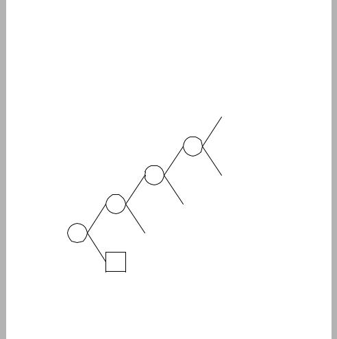
Figure 3.46 Huffman tree for sequence 2 motion vectors
The corresponding Huffman tree is given in Figure 3.46. The ‘shape’ of the tree has changed (because of the distribution of probabilities) and this gives a different set of Huffman codes (shown in Table 3.5). There are still four nodes in the tree, one less than the number of data items (five), as is always the case with Huffman coding.
If the probability distributions are accurate, Huffman coding provides a relatively compact representation of the original data. In these examples, the frequently occurring (0) vector is represented efficiently as a single bit. However, to achieve optimum compression, a separate code table is required for each of the two sequences because of their different probability distributions. The loss of potential compression efficiency due to the requirement for integrallength codes is very clear for vector ‘0’ in sequence 2, since the optimum number of bits (information content) is 0.32 but the best that can be achieved with Huffman coding is 1 bit.
3.5.2.2 Pre-calculated Huffman-based Coding
The Huffman coding process has two disadvantages for a practical video CODEC. First, the decoder must use the same codeword set as the encoder. Transmitting the information contained in the probability table to the decoder would add extra overhead and reduce compression
66 |
|
|
|
|
VIDEO CODING CONCEPTS |
||
|
|
|
|
|
|||
• |
|
Table 3.6 MPEG-4 Visual Transform Coefficient |
|||||
|
(TCOEF) VLCs (partial, all codes <9 bits) |
|
|||||
|
|
|
Last |
Run |
Level |
Code |
|
|
|
|
|
|
|
|
|
|
|
0 |
0 |
1 |
10s |
||
|
|
0 |
1 |
1 |
110s |
||
|
|
0 |
2 |
1 |
1110s |
||
|
|
0 |
0 |
2 |
1111s |
||
|
|
1 |
0 |
1 |
0111s |
||
|
|
0 |
3 |
1 |
01101s |
||
|
|
0 |
4 |
1 |
01100s |
||
|
|
0 |
5 |
1 |
01011s |
||
|
|
0 |
0 |
3 |
010101s |
||
|
|
0 |
1 |
2 |
010100s |
||
|
|
0 |
6 |
1 |
010011s |
||
|
|
0 |
7 |
1 |
010010s |
||
|
|
0 |
8 |
1 |
010001s |
||
|
|
0 |
9 |
1 |
010000s |
||
|
|
1 |
1 |
1 |
001111s |
||
|
|
1 |
2 |
1 |
001110s |
||
|
|
1 |
3 |
1 |
001101s |
||
|
|
1 |
4 |
1 |
001100s |
||
|
|
0 |
0 |
4 |
0010111s |
||
|
|
0 |
10 |
1 |
0010110s |
||
|
|
0 |
11 |
1 |
0010101s |
||
|
|
0 |
12 |
1 |
0010100s |
||
|
|
1 |
5 |
1 |
0010011s |
||
|
|
1 |
6 |
1 |
0010010s |
||
|
|
1 |
7 |
1 |
0010001s |
||
|
|
1 |
8 |
1 |
0010000s |
||
|
|
ESCAPE |
· · · |
· · · |
0000011s |
||
|
|
|
· · · |
· · · |
|
||
efficiency, particularly for shorter video sequences. Second, the probability table for a large video sequence (required to generate the Huffman tree) cannot be calculated until after the video data is encoded which may introduce an unacceptable delay into the encoding process. For these reasons, recent image and video coding standards define sets of codewords based on the probability distributions of ‘generic’ video material. The following two examples of pre-calculated VLC tables are taken from MPEG-4 Visual (Simple Profile).
Transform Coefficients (TCOEF)
MPEG-4 Visual uses 3D coding of quantised coefficients in which each codeword represents a combination of (run, level, last). A total of 102 specific combinations of (run, level, last) have VLCs assigned to them and 26 of these codes are shown in Table 3.6.
A further 76 VLCs are defined, each up to 13 bits long. The last bit of each codeword is the sign bit ‘s’, indicating the sign of the decoded coefficient (0 = positive, 1 = negative). Any (run, level, last) combination that is not listed in the table is coded using an escape sequence, a special ESCAPE code (0000011) followed by a 13-bit fixed length code describing the values of run, level and last.

ENTROPY CODER |
• |
|
67 |
|
|
Table 3.7 MPEG4 Motion Vector
Difference (MVD) VLCs
MVD |
Code |
|
|
0 |
1 |
+0.5 |
010 |
−0.5 |
011 |
+1 |
0010 |
−1 |
0011 |
+1.5 |
00010 |
−1.5 |
00011 |
+2 |
0000110 |
−2 |
0000111 |
+2.5 |
00001010 |
−2.5 |
00001011 |
+3 |
00001000 |
−3 |
00001001 |
+3.5 |
00000110 |
−3.5 |
00000111 |
· · · |
· · · |
Some of the codes shown in Table 3.6 are represented in ‘tree’ form in Figure 3.47. A codeword containing a run of more than eight zeros is not valid, hence any codeword starting with 000000000. . . indicates an error in the bitstream (or possibly a start code, which begins with a long sequence of zeros, occurring at an unexpected position in the sequence). All other sequences of bits can be decoded as valid codes. Note that the smallest codes are allocated to short runs and small levels (e.g. code ‘10’ represents a run of 0 and a level of ±1), since these occur most frequently.
Motion Vector Difference (MVD)
Differentially coded motion vectors (MVD) are each encoded as a pair of VLCs, one for the x-component and one for the y-component. Part of the table of VLCs is shown in Table 3.7. A further 49 codes (8–13 bits long) are not shown here. Note that the shortest codes represent small motion vector differences (e.g. MVD = 0 is represented by a single bit code ‘1’).
These code tables are clearly similar to ‘true’ Huffman codes since each symbol is assigned a unique codeword, common symbols are assigned shorter codewords and, within a table, no codeword is the prefix of any other codeword. The main differences from ‘true’ Huffman coding are (1) the codewords are pre-calculated based on ‘generic’ probability distributions and (b) in the case of TCOEF, only 102 commonly-occurring symbols have defined codewords with any other symbol encoded using a fixed-length code.
3.5.2.3 Other Variable-length Codes
As well as Huffman and Huffman-based codes, a number of other families of VLCs are of potential interest in video coding applications. One serious disadvantage of Huffman-based codes for transmission of coded data is that they are sensitive to transmission errors. An

68 |
|
|
VIDEO CODING CONCEPTS |
|||
|
• |
|
|
|
|
000000000X (error) |
|
|
|
|
|
||
|
|
|
|
|
|
... 4 codes |
|
|
|
|
|
||
... 4 codes
... 8 codes
... 24 codes 0000011 (escape)
0 |
|
|
|
|
|
|
|
|
|
... 17 codes |
||||
|
|
|
|
|
|
|
|
|
||||||
|
|
|
|
|
|
|
|
... 19 codes |
||||||
1 |
|
|
|
|
|
|
||||||||
|
|
|
|
|
|
|||||||||
0 |
|
|
|
|
|
... 12 codes |
||||||||
|
|
|
|
|
||||||||||
|
|
|
|
|
|
|
|
|
|
|
|
|
||
Start |
|
|
|
|
|
|
|
|
|
010000 (0,9,1) |
||||
|
|
|
|
|
|
|||||||||
1 |
|
|
|
|
|
|
|
|
|
010001 (0,8,1) |
||||
|
|
|
|
|
|
|
|
|
|
|
010010 (0,7,1) |
|||
|
|
|
|
|
|
|
|
|
|
|
|
|||
|
|
|
|
|
|
|
|
|
|
|
010011 (0,6,1) |
|||
|
|
|
|
|
|
|
|
|
|
|
|
|
|
010100 (0,1,2) |
|
|
|
|
|
|
|
|
|
|
|
|
|
|
|
|
|
|
|
|
|
|
|
|
|
|
|
|
|
010101 (0,0,3) |
|
|
|
|
|
|
|
|
|
|
|
|
|
|
|
|
|
|
|
|
|
|
|
|
|
|
|
01011 (0,5,1) |
||
|
|
|
|
|
|
|
|
|
|
|
|
|||
|
|
|
|
|
|
|
|
|
|
|
|
|
01100 (0,4,1) |
|
|
|
|
|
|
|
|
|
|
|
|
|
|
||
|
|
|
|
|
|
|
|
|
|
|
|
|
01101 (0,3,1) |
|
|
|
|
|
|
|
|
|
|
|
|
|
|
||
|
|
|
|
|
|
|
|
|
0111 (1,0,1) |
|
||||
|
|
|
|
|
|
|
|
|
||||||
010 (0,0,1)
|
|
|
|
|
|
110 (0,1,1) |
|||
|
|
|
|
||||||
1 |
|
|
|
|
|
|
1110 (0,2,1) |
||
|
|
|
|
|
|
|
|
|
|
1111 (0,0,2)
Figure 3.47 MPEG4 TCOEF VLCs (partial)
error in a sequence of VLCs may cause a decoder to lose synchronisation and fail to decode subsequent codes correctly, leading to spreading or propagation of an error in a decoded sequence. Reversible VLCs (RVLCs) that can be successfully decoded in either a forward or a backward direction can improve decoding performance when errors occur (see Section 5.3). A drawback of pre-defined code tables (such as Table 3.6 and Table 3.7) is that both encoder and decoder must store the table in some form. An alternative approach is to use codes that