

• |
VIDEO CODING CONCEPTS |
42 |
Reference frame
Possible |
matching |
positions |
Current frame
Problematic |
macroblock |
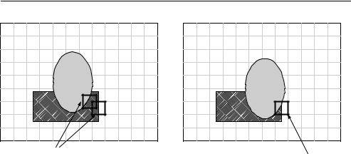
Figure 3.23 Motion compensation of arbitrary-shaped moving objects
oval-shaped object is moving and the rectangular object is static. It is difficult to find a good match in the reference frame for the highlighted macroblock, because it covers part of the moving object and part of the static object. Neither of the two matching positions shown in the reference frame are ideal.
It may be possible to achieve better performance by motion compensating arbitrary regions of the picture (region-based motion compensation). For example, if we only attempt to motion-compensate pixel positions inside the oval object then we can find a good match in the reference frame. There are however a number of practical difficulties that need to be overcome in order to use region-based motion compensation, including identifying the region boundaries accurately and consistently, (segmentation) signalling (encoding) the contour of the boundary to the decoder and encoding the residual after motion compensation. MPEG-4 Visual includes a number of tools that support region-based compensation and coding and these are described in Chapter 5.
3.4 IMAGE MODEL
A natural video image consists of a grid of sample values. Natural images are often difficult to compress in their original form because of the high correlation between neighbouring image samples. Figure 3.24 shows the two-dimensional autocorrelation function of a natural video image (Figure 3.4) in which the height of the graph at each position indicates the similarity between the original image and a spatially-shifted copy of itself. The peak at the centre of the figure corresponds to zero shift. As the spatially-shifted copy is moved away from the original image in any direction, the function drops off as shown in the figure, with the gradual slope indicating that image samples within a local neighbourhood are highly correlated.
A motion-compensated residual image such as Figure 3.20 has an autocorrelation function (Figure 3.25) that drops off rapidly as the spatial shift increases, indicating that neighbouring samples are weakly correlated. Efficient motion compensation reduces local correlation in the residual making it easier to compress than the original video frame. The function of the image
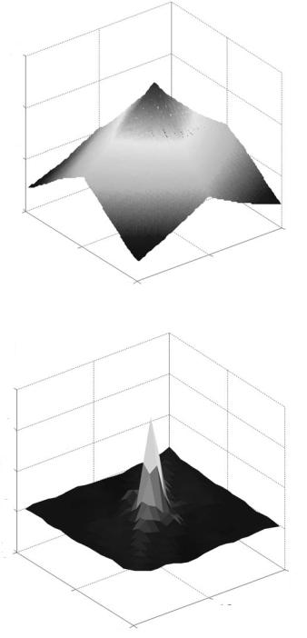
IMAGE MODEL |
• |
|
43 |
|
|
X 108
8
6
4
2
100
100
50
50
00
Figure 3.24 2D autocorrelation function of image
X 105
6
4
2
0
 −2 20
−2 20
20
10
10
00
Figure 3.25 2D autocorrelation function of residual

• |
VIDEO CODING CONCEPTS |
44 |
|
Raster |
|
scan |
|
order |
B |
C |
A X
Current pixel
Figure 3.26 Spatial prediction (DPCM)
model is to decorrelate image or residual data further and to convert it into a form that can be efficiently compressed using an entropy coder. Practical image models typically have three main components, transformation (decorrelates and compacts the data), quantisation (reduces the precision of the transformed data) and reordering (arranges the data to group together significant values).
3.4.1 Predictive Image Coding
Motion compensation is an example of predictive coding in which an encoder creates a prediction of a region of the current frame based on a previous (or future) frame and subtracts this prediction from the current region to form a residual. If the prediction is successful, the energy in the residual is lower than in the original frame and the residual can be represented with fewer bits.
In a similar way, a prediction of an image sample or region may be formed from previously-transmitted samples in the same image or frame. Predictive coding was used as the basis for early image compression algorithms and is an important component of H.264 Intra coding (applied in the transform domain, see Chapter 6). Spatial prediction is sometimes described as ‘Differential Pulse Code Modulation’ (DPCM), a term borrowed from a method of differentially encoding PCM samples in telecommunication systems.
Figure 3.26 shows a pixel X that is to be encoded. If the frame is processed in raster order, then pixels A, B and C (neighbouring pixels in the current and previous rows) are available in both the encoder and the decoder (since these should already have been decoded before X). The encoder forms a prediction for X based on some combination of previously-coded pixels, subtracts this prediction from X and encodes the residual (the result of the subtraction). The decoder forms the same prediction and adds the decoded residual to reconstruct the pixel.
Example
Encoder prediction P(X) = (2A + B + C)/4
Residual R(X) = X – P(X) is encoded and transmitted.
Decoder decodes R(X) and forms the same prediction: P(X) = (2A + B + C)/4 Reconstructed pixel X = R(X) + P(X)
IMAGE MODEL |
• |
|
45 |
|
|
If the encoding process is lossy (e.g. if the residual is quantised – see section 3.4.3) then the decoded pixels A , B and C may not be identical to the original A, B and C (due to losses during encoding) and so the above process could lead to a cumulative mismatch (or ‘drift’) between the encoder and decoder. In this case, the encoder should itself decode the residual R (X) and reconstruct each pixel.
The encoder uses decoded pixels A , B and C to form the prediction, i.e. P(X) = (2A + B + C )/4 in the above example. In this way, both encoder and decoder use the same prediction P(X) and drift is avoided.
The compression efficiency of this approach depends on the accuracy of the prediction P(X). If the prediction is accurate (P(X) is a close approximation of X) then the residual energy will be small. However, it is usually not possible to choose a predictor that works well for all areas of a complex image and better performance may be obtained by adapting the predictor depending on the local statistics of the image (for example, using different predictors for areas of flat texture, strong vertical texture, strong horizontal texture, etc.). It is necessary for the encoder to indicate the choice of predictor to the decoder and so there is a tradeoff between efficient prediction and the extra bits required to signal the choice of predictor.
3.4.2 Transform Coding
3.4.2.1 Overview
The purpose of the transform stage in an image or video CODEC is to convert image or motion-compensated residual data into another domain (the transform domain). The choice of transform depends on a number of criteria:
1.Data in the transform domain should be decorrelated (separated into components with minimal inter-dependence) and compact (most of the energy in the transformed data should be concentrated into a small number of values).
2.The transform should be reversible.
3.The transform should be computationally tractable (low memory requirement, achievable using limited-precision arithmetic, low number of arithmetic operations, etc.).
Many transforms have been proposed for image and video compression and the most popular transforms tend to fall into two categories: block-based and image-based. Examples of block-based transforms include the Karhunen–Loeve Transform (KLT), Singular Value Decomposition (SVD) and the ever-popular Discrete Cosine Transform (DCT) [3]. Each of these operate on blocks of N × N image or residual samples and hence the image is processed in units of a block. Block transforms have low memory requirements and are well-suited to compression of block-based motion compensation residuals but tend to suffer from artefacts at block edges (‘blockiness’). Image-based transforms operate on an entire image or frame (or a large section of the image known as a ‘tile’). The most popular image transform is the Discrete Wavelet Transform (DWT or just ‘wavelet’). Image transforms such as the DWT have been shown to out-perform block transforms for still image compression but they tend to have higher memory requirements (because the whole image or tile is processed as a unit) and
• |
VIDEO CODING CONCEPTS |
46 |
do not ‘fit’ well with block-based motion compensation. The DCT and the DWT both feature in MPEG-4 Visual (and a variant of the DCT is incorporated in H.264) and are discussed further in the following sections.
3.4.2.2 DCT
The Discrete Cosine Transform (DCT) operates on X, a block of N × N samples (typically image samples or residual values after prediction) and creates Y, an N × N block of coefficients. The action of the DCT (and its inverse, the IDCT) can be described in terms of a transform matrix A. The forward DCT (FDCT) of an N × N sample block is given by:
Y = AXAT |
(3.1) |
and the inverse DCT (IDCT) by: |
|
X = ATYA |
(3.2) |
where X is a matrix of samples, Y is a matrix of coefficients and A is an N × N transform matrix. The elements of A are:
|
i j = |
i |
|
2N |
i = |
|
|
N |
|
= |
|
|
i = |
|
|
N |
|
|||
A |
|
C |
cos |
(2 j + 1)i π |
where C |
|
|
|
1 |
(i |
|
0), |
C |
|
|
|
2 |
(i > 0) (3.3) |
||
|
|
|
|
|
|
|
||||||||||||||
Equation 3.1 and equation 3.2 may be written in summation form:
Y |
|
|
C C |
N −1 N −1 |
X |
|
cos (2 j + 1)yπ cos (2i + 1)xπ |
(3.4) |
|||
|
x y = |
|
|
|
|
|
|
|
|
|
|
|
x |
y |
|
i j |
|
2N |
|
2N |
|
||
|
|
|
|
i =0 j =0 |
|
|
|
|
|
|
|
X |
|
N −1 N −1 C C Y |
|
cos (2 j + 1)yπ cos (2i + 1)xπ |
(3.5) |
||||||
|
|
i j = |
|
|
|
|
|
|
|
|
|
|
|
x=0 |
x y x y |
|
2N |
|
2N |
|
|||
|
|
|
y=0 |
|
|
|
|
|
|
|
|
Example: N = 4
The transform matrix A for a 4 × 4 DCT is: |
|
|
|
|
|
|
|
|
|
|
|
|
|
|
|
|
|
|
|
|
|
|
|||||||||||||||||||||||
|
|
|
|
|
1 |
|
|
|
|
|
|
|
1 |
|
|
|
|
1 |
|
|
|
|
|
1 |
|
|
|
|
|
|
|||||||||||||||
|
|
|
|
|
|
|
|
|
cos (0) |
|
|
|
|
|
cos (0) |
|
|
|
|
|
|
|
cos (0) |
|
|
|
|
|
|
|
cos (0) |
|
|||||||||||||
|
|
|
|
|
|
2 |
|
|
2 |
|
|
2 |
|
2 |
|
||||||||||||||||||||||||||||||
|
|
|
|
|
|
|
|
|
|
|
|
|
|
|
|
|
|
|
|
|
|
|
|
|
|
|
|
|
|
|
|
|
|
|
|
|
|
|
|
|
|
||||
|
|
|
|
|
|
1 |
cos |
|
π |
|
|
|
1 |
cos |
3π |
|
|
|
|
1 |
cos |
|
|
5π |
|
|
|
1 |
cos |
|
|
7π |
|
||||||||||||
|
|
|
|
|
|
|
|
|
|
|
|
|
|
|
|
|
|
|
|
|
|
|
|
|
|
|
|
||||||||||||||||||
|
|
|
|
|
2 |
|
8 |
|
|
|
|
|
8 |
|
|
2 |
8 |
|
|
|
8 |
|
|||||||||||||||||||||||
|
|
|
|
|
|
|
|
|
|
2 |
|
|
|
|
|
|
|
|
2 |
|
|
|
|
||||||||||||||||||||||
|
|
|
|
|
|
|
|
|
|
|
|
|
|
|
|
|
|
|
|
|
|
|
|
|
|
|
|
|
|||||||||||||||||
A |
= |
|
|
|
|
|
|
|
|
|
|
|
|
|
|
|
|
|
|
|
|
|
|
|
|
|
|
|
|
|
|
|
|
|
|
|
(3.6) |
||||||||
|
|
|
1 |
|
|
|
|
2π |
|
1 |
|
|
6π |
|
1 |
|
|
|
|
10π |
|
1 |
|
|
|
|
14π |
|
|
||||||||||||||||
|
|
|
2 |
|
|
|
|
8 |
|
2 |
|
|
8 |
2 |
|
|
|
8 |
2 |
|
|
|
|
8 |
|
|
|||||||||||||||||||
|
|
|
|
|
|
|
|
|
|
|
|
|
|
|
|
|
|
|
|
|
|
|
|
|
|
|
|
||||||||||||||||||
|
|
|
|
|
|
|
cos |
|
|
|
|
|
|
|
cos |
|
|
|
|
|
|
|
cos |
|
|
|
|
|
|
|
|
cos |
|
|
|
|
|
||||||||
|
|
|
|
|
|
|
|
|
|
|
|
|
|
|
|
|
|
|
|
|
|
|
|
|
|
|
|
|
|
|
|
|
|
||||||||||||
|
|
|
|
|
|
|
|
|
|
|
|
|
|
|
|
|
|
|
|
|
|
|
|
|
|
|
|
|
|
|
|
|
|
|
|
|
|
|
|
|
|
|
|
|
|
|
|
|
|
|
|
|
|
|
|
|
|
|
|
|
|
|
|
|
|
|
|
|
|
|
|
|
|
|
|
|
|
|
|
||||||||||||
|
|
|
1 |
|
|
|
|
3π |
|
1 |
|
|
9π |
|
1 |
|
|
|
|
15π |
|
1 |
|
|
|
|
21π |
|
|||||||||||||||||
|
|
|
2 |
|
|
|
|
8 |
|
2 |
|
|
8 |
2 |
|
|
|
8 |
2 |
|
|
|
|
8 |
|
|
|||||||||||||||||||
|
|
|
|
|
|
|
|
|
|
|
|
|
|
|
|
|
|
|
|
|
|
|
|
|
|
|
|
||||||||||||||||||
|
|
|
|
|
|
|
cos |
|
|
|
|
|
|
|
cos |
|
|
|
|
|
|
|
cos |
|
|
|
|
|
|
|
|
cos |
|
|
|
|
|
||||||||

IMAGE MODEL |
|
|
|
|
|
|
|
|
|
|
|
|
|
|
|
|
|
|
|
|
|
|
|
|
|
|
|
|
|
|
|
|
|
|
|
|
|
|
|
|
|
|
|
|
|
|
|
|
|
|
|
|
|
|
|
|
|
|
|
|
|
|
|
|
|
|
|
|
|
|
|
47 |
|
||||||
|
|
|
|
|
|
|
|
|
|
|
|
|
|
|
|
|
|
|
|
|
|
|
|
|
|
|
|
|
|
|
|
|
|
|
|
|
|
|
|
|
|
|
|
|
|
|
|
|
|
|
|
|
|
|
|
|
|
|
|||||||||||||||||||||
|
The cosine function is symmetrical and repeats after 2π |
|
|
|
|
|
|
|
|
|
|
|
|
hence A can be simplified |
|||||||||||||||||||||||||||||||||||||||||||||||||||||||||||||||||
|
to: |
|
|
|
|
|
|
|
1 |
|
|
|
|
|
|
|
|
|
|
|
|
|
|
|
|
1 |
|
|
|
|
|
|
|
|
|
|
|
|
|
1 |
|
|
|
radians and |
|
|
|
|
|
|
1 |
|
|
|
|
|
|
• |
|
||||||||||||||||||||
|
|
|
|
|
|
|
|
|
|
|
|
|
|
|
|
|
|
|
|
|
|
|
|
|
|
|
|
|
|
|
|
|
|
|
|
|
|
|
|
|
|
|
|
|
|
|
|
|
|
|
|
|
|
|
|
|
|
|
|
|
|
|
|
|
|
|
|
|
|
|
|
|
|
|
|
|
|||
|
|
|
|
|
|
|
|
2 |
|
|
|
π |
|
|
|
|
|
|
|
|
|
|
|
2 |
|
|
|
3π |
|
|
|
|
|
|
|
|
2 |
|
|
3π |
|
|
|
|
|
|
|
|
|
|
|
|
|
|
2 |
|
|
|
π |
|
|
|
|
||||||||||||||||
|
|
|
|
|
1 cos |
|
|
|
|
|
|
|
1 cos |
|
|
|
|
|
|
|
|
1 cos |
|
|
|
|
|
|
|
|
|
|
|
1 cos |
|
|
|
|
|
||||||||||||||||||||||||||||||||||||||||
|
|
|
|
|
|
|
|
|
|
|
|
|
|
|
|
|
|
|
|
|
|
|
|
|
|
|
|
|
|
|
|
|
|
|
|
|
|
− |
|
|
|
|
|
|
|
|
|
|
|
|
|
|
|
− |
|
|
|
|
|
|
|
|
|
|
|
|
|
|
|
|
|
||||||||
|
A |
|
|
2 |
|
|
|
|
|
8 |
|
|
|
2 |
|
|
|
|
|
|
|
|
8 |
|
|
2 |
|
|
|
|
|
|
8 |
|
|
|
|
|
2 |
|
|
|
|
|
|
8 |
|
(3.7) |
|
|
|||||||||||||||||||||||||||||
|
|
|
|
|
|
|
|
|
|
|
|
|
|
|
|
|
|
|
|
|
|
|
|
|
|
|
|
|
|
|
|
|
|
|
|
|
|
|
|
|
|
|
|
|
|
|
|
|
|
|
|
|
|
|
|
|
|
|
|
|
|
|
|
|
|
|
|
|
|
|
|
|
|
|
|
|
|
|
|
|
|
= |
|
|
|
|
|
1 |
|
|
|
|
|
|
|
|
|
|
|
|
|
|
|
|
|
|
|
1 |
|
|
|
|
|
|
|
|
|
|
|
|
|
1 |
|
|
|
|
|
|
|
|
|
|
|
|
|
|
|
|
|
|
|
|
1 |
|
|
|
|
|
|
|
|
|
|||||||
|
|
|
|
|
|
|
|
|
|
|
|
|
|
|
|
|
|
|
|
|
|
|
|
|
|
|
|
− |
|
|
|
|
|
|
|
|
|
|
|
|
− |
|
|
|
|
|
|
|
|
|
|
|
|
|
|
|
|
|
|
|
|
|
|
|
|
|
|
|
|
|
|
|
|
|
|
||||
|
|
|
|
|
|
|
|
2 |
|
|
|
|
|
|
|
|
|
|
|
|
|
|
|
|
2 |
|
|
|
|
|
|
|
|
|
|
|
2 |
|
|
|
|
|
|
|
|
|
|
|
|
|
|
|
|
|
|
|
|
2 |
|
|
|
|
|
|
|
|
|
||||||||||||
|
|
|
|
|
|
|
|
|
|
|
|
|
|
|
|
|
|
|
|
|
|
|
|
|
|
|
|
|
|
|
|
|
|
|
|
|
|
|
|
|
|
|
|
|
|
|
|
|
|
|
|
|
|
|
|
|
|
|
|
|
|
|
|
|
|
|
|
|
|
|
|
|
|
|
|
|
|
|
|
|
|
|
|
|
|
|
|
|
|
|
|
|
|
|
|
|
|
|
|
|
|
|
|
|
|
|
|
|
|
|
|
|
|
|
|
|
|
|
|
|
|
|
|
|
|
|
|
|
|
|
|
|
|
|
|
|
|
|
|
|
|
|
|
|
|
|
|
|
|
|
|
|
|
|
|
|
|
|
|
|
|
|
|
1 |
|
|
|
|
|
3π |
|
|
|
1 |
|
|
|
|
|
|
π |
|
|
|
|
|
1 |
|
|
|
|
|
π |
|
|
|
|
|
|
|
|
|
1 |
|
|
|
|
|
|
|
3π |
|
|
|
|
||||||||||||||||||||||||
|
|
|
|
|
|
|
|
|
|
|
|
|
|
|
|
|
|
|
|
|
|
|
|
|
|
|
|
|
|
|
|
|
|
|
|
|
|
|
|
|
|
|
|
|
|
|
|
|
|
|
|
|
|
|
|
|
|
|
|
|
|
|
|
|
|
|
|
|
|
|
|
|
|
|
|
|
|
|
|
|
|
|
|
|
|
|
|
|
|
|
|
|
− |
|
|
|
|
|
|
|
|
|
|
|
|
|
|
|
|
|
|
|
|
|
|
|
|
|
− |
|
|
|
|
|
|
|
|
|
|
|
|
|
|
|
|
|
|||||||||||||||||||||||
|
or |
|
|
2 |
8 |
|
|
|
|
2 |
|
|
8 |
|
|
2 |
|
|
|
8 |
|
|
|
|
2 |
|
|
|
|
8 |
|
|
|
|
|||||||||||||||||||||||||||||||||||||||||||||
|
|
|
|
|
|
|
cos |
|
|
|
|
|
|
|
|
|
|
|
|
|
|
|
|
cos |
|
|
|
|
|
|
|
|
|
|
|
|
|
|
|
|
|
|
|
|
|
|
|
cos |
|
|
|
|
|
|
|||||||||||||||||||||||||
|
|
|
|
|
|
|
|
|
|
|
|
|
|
|
|
|
|
|
|
|
|
|
|
|
|
|
|
|
|
|
|
|
|
cos |
|
|
|
|
|
|
|
|
|
|
|
|
|
|
|
|
|
|
|
|
|
|
|
|
|||||||||||||||||||||
|
|
|
|
|
|
|
|
|
|
|
|
|
|
|
|
|
|
|
|
|
|
|
|
|
|
|
|
|
|
|
|
|
|
|
|
|
|
|
|
|
|
|
|
|
|
|
|
|
|
|
|
|
|
a = |
1 |
|
|
|
|
|
|
|
|
|
|
|
|
|
|
|
|
|
|||||||
|
|
|
|
|
|
|
|
|
|
|
|
|
|
|
|
|
|
|
|
|
|
|
|
|
|
|
|
|
|
|
|
|
|
|
|
|
|
|
|
|
|
|
|
|
|
|
|
|
|
|
|
|
|
|
|
|
|
|
|
|
|
|
|
|
|
|
|
|
|
|
|
||||||||
|
|
|
|
|
|
|
|
|
|
|
|
|
|
A |
|
|
|
b |
|
|
|
|
|
c |
−c |
|
−b |
where |
|
|
b |
|
|
2 |
|
|
|
|
|
π |
|
|
|
|
|
(3.8) |
|
|
|||||||||||||||||||||||||||||||
|
|
|
|
|
|
|
|
|
|
|
|
|
|
|
|
|
|
|
|
|
|
|
|
|
|
|
|
|
|
1 cos |
|
|
|
|
|
|
|
||||||||||||||||||||||||||||||||||||||||||
|
|
|
|
|
|
|
|
|
|
|
|
|
|
|
|
|
|
|
|
|
a |
|
|
|
|
|
a |
|
|
|
a |
|
|
a |
|
|
|
|
|
|
|
|
|
|
|
|
|
|
|
|
|
|
|
|
|
|
|
|
|
|
|
|
|
|
|
|
|
|
|
|
|
|
|
|
|||||
|
|
|
|
|
|
|
|
|
|
|
|
|
|
|
|
|
= |
|
a |
|
|
|
|
|
a |
|
|
|
a |
|
|
a |
|
|
|
|
|
|
|
|
|
|
|
= |
2 |
|
|
|
|
|
|
8 |
|
|
|
|
|
|
|
|
|
||||||||||||||||||
|
|
|
|
|
|
|
|
|
|
|
|
|
|
|
|
|
|
|
|
c |
|
− |
|
|
|
|
− |
|
|
|
|
|
|
|
|
|
|
|
|
|
|
|
|
|
|
|
|
|
|
|
|
|
|
|
|
|
|
|
|
|
|
|
|
||||||||||||||||
|
|
|
|
|
|
|
|
|
|
|
|
|
|
|
|
|
|
|
|
|
|
|
|
|
b |
|
|
|
b |
|
|
c |
|
|
|
|
|
|
|
|
|
|
|
|
|
|
|
|
|
|
|
|
|
|
|
|
|
|
|
|
|
|
|
|
|
|
|
|
|
|
|||||||||
|
|
|
|
|
|
|
|
|
|
|
|
|
|
|
|
|
|
|
|
|
|
|
|
|
|
|
|
|
|
|
|
|
|
|
|
|
|
|
|
|
|
1 |
|
|
|
|
|
|
|
|
|
|
3π |
|
|
|
|
|
|
|
|
||||||||||||||||||
|
|
|
|
|
|
|
|
|
|
|
|
|
|
|
|
|
|
|
|
|
|
|
|
− |
|
|
|
|
|
|
|
|
|
|
|
|
|
|
|
|
|
|
|
|
|
|
|
|
|
|
|
|
|
|
|
|
|
|
|
|
|
|
|
|
|
|
|
||||||||||||
|
|
|
|
|
|
|
|
|
|
|
|
|
|
|
|
|
|
|
|
|
|
|
|
|
|
|
|
|
|
|
|
|
|
|
|
|
|
|
|
|
|
|
c |
|
|
|
|
|
|
cos |
|
|
|
|
|
|
|
|
|
|
|
|
|
|
|
|
|
|
|||||||||||
|
|
|
|
|
|
|
|
|
|
|
|
|
|
|
|
|
|
|
|
|
|
|
|
|
|
|
|
|
|
|
|
|
|
|
|
|
|
|
|
|
|
|
|
|
= |
2 |
|
|
8 |
|
|
|
|
|
|
|
|
|
|||||||||||||||||||||
|
Evaluating the cosines gives: |
|
|
|
|
|
|
|
|
|
|
|
|
|
|
|
|
|
|
|
|
|
|
|
|
|
|
|
|
|
|
|
|
|
|
||||||||||||||||||||||||||||||||||||||||||||
|
|
|
|
|
|
|
|
|
|
|
|
|
|
|
|
|
|
|
|
|
|
|
−0.653 |
|
|
|
|
|
|
|
|
|
|
|
|
|
|||||||||||||||||||||||||||||||||||||||||||
|
|
|
|
|
|
|
|
|
|
|
|
|
|
|
|
|
|
|
|
A |
|
|
|
0.653 |
|
0.271 |
|
0.271 |
|
|
|
|
|
|
|
|
|
|
|
|
|
|
|
|
|||||||||||||||||||||||||||||||||||
|
|
|
|
|
|
|
|
|
|
|
|
|
|
|
|
|
|
|
|
|
|
|
|
|
0.5 |
|
|
|
|
|
0.5 |
|
|
|
|
0.5 |
|
|
|
|
|
|
0.5 |
|
|
|
|
|
|
|
|
|
|
|
|
|
|
||||||||||||||||||||||
|
|
|
|
|
|
|
|
|
|
|
|
|
|
|
|
|
|
|
|
|
|
= |
|
0.271 |
|
|
|
0.653 |
|
|
|
|
0.653 |
|
|
|
0.271 |
|
|
|
|
|
|
|
|
|
|
|
|
|
|||||||||||||||||||||||||||||
|
|
|
|
|
|
|
|
|
|
|
|
|
|
|
|
|
|
|
|
|
|
|
|
0.5 |
|
|
|
|
−0.5 |
|
|
−0.5 |
|
|
|
|
0.5 |
|
|
|
|
|
|
|
|
|
|
|
|
|
|
||||||||||||||||||||||||||||
|
|
|
|
|
|
|
|
|
|
|
|
|
|
|
|
|
|
|
|
|
|
|
|
|
|
|
|
|
|
|
|
|
|
− |
|
|
|
|
− |
|
|
|
|
|
|
|
|
|
|
|
|
|
|
|
|
|
|
|
|
|
|
|
|
|
|
|
|
||||||||||||
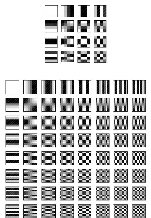
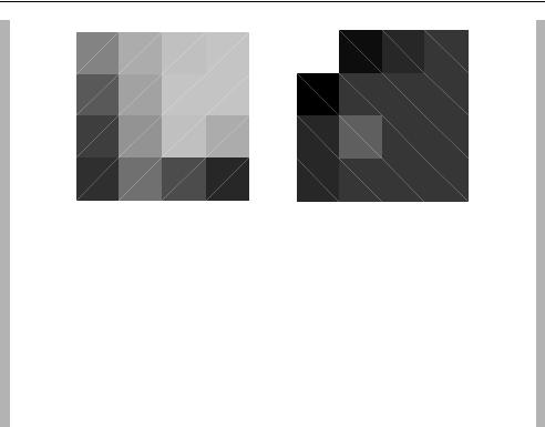
The output of a two-dimensional FDCT is a set of N × N coefficients representing the image block data in the DCT domain and these coefficients can be considered as ‘weights’ of a set of standard basis patterns. The basis patterns for the 4 × 4 and 8 × 8 DCTs are shown in Figure 3.27 and Figure 3.28 respectively and are composed of combinations of horizontal and vertical cosine functions. Any image block may be reconstructed by combining all N × N basis patterns, with each basis multiplied by the appropriate weighting factor (coefficient).
Example 1 Calculating the DCT of a 4 × 4 block
X is 4 × 4 block of samples from an image:
|
j |
= 0 |
1 |
2 |
3 |
i = 0 |
|
5 |
11 |
8 |
10 |
|
|
|
|
|
|
1 |
|
9 |
8 |
4 |
12 |
|
|
|
|
|
|
2 |
|
1 |
10 |
11 |
4 |
|
|
|
|
|
|
3 |
|
19 |
6 |
15 |
7 |
|
|
|
|
|
|
• |
VIDEO CODING CONCEPTS |
48 |
Figure 3.27 4 × 4 DCT basis patterns
Figure 3.28 8 × 8 DCT basis patterns
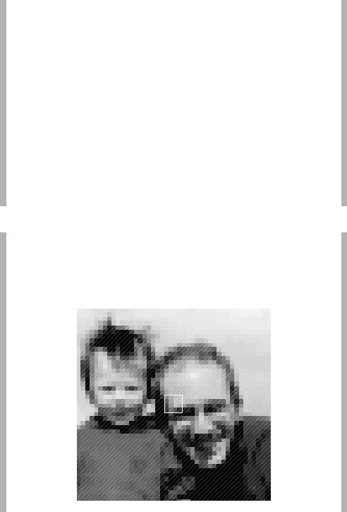
IMAGE MODEL |
• |
|
49 |
|
|
The Forward DCT of X is given by: Y = AXAT . The first matrix multiplication, Y = AX, corresponds to calculating the one-dimensional DCT of each column of X. For example, Y 00 is calculated as follows:
Y00 = A00 X00 + A01 X10 + A02 X20 + A03 X30 = (0.5 5) + (0.5 9) + (0.5 1)
+ (0.5 19) = 17.0
The complete result of the column calculations is:
Y AX |
−6.981 |
2.725 |
−6.467 |
|
4.125 |
|
|||
|
|
|
17 |
17.5 |
19 |
|
16.5 |
|
|
= = |
|
9.015 |
2.660 |
2.679 |
|
4.414 |
|||
|
|
7 |
−0.5 |
4 |
|
0.5 |
|
||
|
− |
− |
|
||||||
|
|
|
|
|
|||||
Carrying out the second matrix multiplication, Y = Y AT , is equivalent to carrying out a 1-D DCT on each row of Y :
Y AXAT |
|
−3.299 |
−4.768 |
|
0.443 |
−9.010 |
|
|||
|
|
|
|
35.0 |
−0.079 |
|
−1.5 |
1.115 |
|
|
= |
= |
|
4.045 |
|
3.010 |
|
9.384 |
1.232 |
||
|
|
|
|
5.5 |
|
3.029 |
|
2.0 |
4.699 |
|
|
|
|
− |
|
− |
|
− |
|
− |
|
(Note: the order of the row and column calculations does not affect the final result).
Example 2 Image block and DCT coefficients
Figure 3.29 shows an image with a 4 × 4 block selected and Figure 3.30 shows the block in close-up, together with the DCT coefficients. The advantage of representing the block in the DCT domain is not immediately obvious since there is no reduction in the amount of data; instead of 16 pixel values, we need to store 16 DCT coefficients. The usefulness of the DCT becomes clear when the block is reconstructed from a subset of the coefficients.
Figure 3.29 Image section showing 4 × 4 block
50 |
|
|
|
|
|
|
VIDEO CODING CONCEPTS |
|
• |
126 |
159 |
178 |
181 |
537.2 |
-76.0 -54.8 -7.8 |
||
|
98 |
151 |
181 |
181 |
-106.1 |
35.0 |
-12.7 |
-6.1 |
|
80 |
137 |
176 |
156 |
-42.7 |
46.5 |
10.3 |
-9.8 |
|
75 |
114 |
88 |
68 |
-20.2 |
12.9 |
3.9 |
-8.5 |
|
|
Original block |
|
|
DCT coefficients |
|
||
Figure 3.30 Close-up of 4 × 4 block; DCT coefficients
Setting all the coefficients to zero except the most significant (coefficient 0,0, described as the ‘DC’ coefficient) and performing the IDCT gives the output block shown in Figure 3.31(a), the mean of the original pixel values. Calculating the IDCT of the two most significant coefficients gives the block shown in Figure 3.31(b). Adding more coefficients before calculating the IDCT produces a progressively more accurate reconstruction of the original block and by the time five coefficients are included (Figure 3.31(d)), the reconstructed block is a reasonably close match to the original. Hence it is possible to reconstruct an approximate copy of the block from a subset of the 16 DCT coefficients. Removing the coefficients with insignificant magnitudes (for example by quantisation, see Section 3.4.3) enables image data to be represented with a reduced number of coefficient values at the expense of some loss of quality.
3.4.2.3 Wavelet
The popular ‘wavelet transform’ (widely used in image compression is based on sets of filters with coefficients that are equivalent to discrete wavelet functions [4]. The basic operation of a discrete wavelet transform is as follows, applied to a discrete signal containing N samples. A pair of filters are applied to the signal to decompose it into a low frequency band (L) and a high frequency band (H). Each band is subsampled by a factor of two, so that the two frequency bands each contain N/2 samples. With the correct choice of filters, this operation is reversible.
This approach may be extended to apply to a two-dimensional signal such as an intensity image (Figure 3.32). Each row of a 2D image is filtered with a low-pass and a high-pass filter (Lx and Hx ) and the output of each filter is down-sampled by a factor of two to produce the intermediate images L and H. L is the original image low-pass filtered and downsampled in the x-direction and H is the original image high-pass filtered and downsampled in the x- direction. Next, each column of these new images is filtered with lowand high-pass filters (Ly and Hy ) and down-sampled by a factor of two to produce four sub-images (LL, LH, HL and HH). These four ‘sub-band’ images can be combined to create an output image with the same number of samples as the original (Figure 3.33). ‘LL’ is the original image, low-pass filtered in horizontal and vertical directions and subsampled by a factor of 2. ‘HL’ is high-pass filtered in the vertical direction and contains residual vertical frequencies, ‘LH’ is high-pass filtered in the horizontal direction and contains residual horizontal frequencies and ‘HH’ is high-pass filtered in both horizontal and vertical directions. Between them, the four subband