Добавил:

Andrey Опубликованный материал нарушает ваши авторские права? Сообщите нам.

Вуз:

Санкт-Петербургский государственный электротехнический университет "ЛЭТИ"

Предмет:

Электротехника

Файл:

Jack H.Dynamic system modeling and control.2004.pdf

Скачиваний:

Добавлен:

23.08.2013

Размер:

5.61 Mб

Скачать

☆

<<< < Предыдущая 18 19 20 21 22 23 24 25 26 27 28 2930 / 21730 31 32 33 34 35 36 37 38 39 40 41 42 > Следующая >>>

numerical methods - 4.39

The order of the polynomial should match the number of points. Although, as the number of points increases, the shape of the curve will become less smooth. A common way for dealing with this problem is to fit the spline to a smaller number of points and then verify that it matches the remaining points, or use a least squares method to find the best approximation.

4.6.4 Non-Linear Elements

Despite our deepest wishes for simplicity, most systems contain non-linear components. In the last chapter we looked at dealing with non-linearities by linearizing them locally. Numerical techniques will handle non-linearities easily, but smaller time steps are required for accuracy.

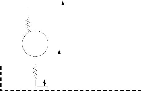
Consider the mass and an applied force shown in Figure 4.39. As the mass moves an aerodynamic resistance force is generated that is proportional to the square of the velocity. This results in a non-linear differential equation. This equation can be numerically integrated using a technique such as Runge-Kutta. Note that the state equation matrix form cannot be used because it requires linear equations.

··

20x

∑Fx

= F – 20x = Mx

(1)

x = v

–20 2

(2)

= --------v

+ ----

Figure 4.39 Developing state equations for a non-linear system

4.7 CASE STUDY

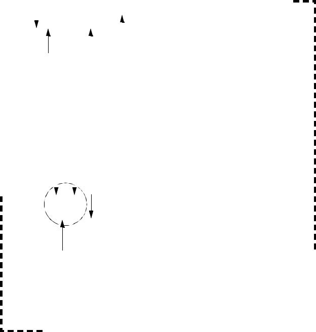
Consider the simplified model of a car suspension shown in Figure 4.40. The model distributes the vehicle weight over four tires with identical suspensions, so the mass of the vehicle is divided by four. In this model the height of the road will change and drive the tire up, or allow it to drop down. The tire acts as a stiff spring, with little deflection. The upper spring and damper are the vibration isolation units. The damper has been designed to stiffen as the damper is compressed. The given table shows how the damping

numerical methods - 4.40

coefficient varies with the amount of compression.

= 50000

---

Ks2

= 200000---

Ks1

= 400Kg

= 20Kg

Ks2

Figure 4.40 A model of a car suspension system


L = yc – yt




	L	Kd



	(cm)	(Ns/m)





30		1000


0		1600
0		1600
-20		2000
-20		2000
-30		2250
-30		2250

For our purposes we will focus only on the translation of the tire, and ignore its rotational motion. The differential equations describing the system are developed in Figure 4.41.

numerical methods - 4.41

··

Mcyc

( y

– y )

( y·

– y·

)

∑F = Ks1( yt – yc) + Kd( yt

– yc) – Mcg = Mcyc

y··

= ( K ) y

+ ( –K ) y

+ ( K ) y·

+ ( –K ) y·

– M

d t

d c

----y

= v

----y

= v

–K

y +

v +

v + ( –g)

v =

---------

------------

---------

-------

Ks1( yt – yc)

Kd( yt

– yc)

··

Mt Mtyt

Ks2( yr – yt)

(1)

(2)

(3)

··

∑F = Ks2( yr – yt) – Ks1( yt – yc) – Kd( yt – yc) – Mtg = Mtyt

··

Mtyt

( Ks2) yr + ( –Ks2 – Ks1) yt + ( Ks1) yc + ( –Kd) yt

(

Kd) yc

– Mtg

–K

– K

–K

y +

v +

v + ( –g)

(4)

---------

----------------------------

---------

------

Figure 4.41 Differential and state equations for the car suspension system

The damping force must be converted from a tabular form to equation form. This is done in Figure 4.42.

numerical methods - 4.42


There are four data points, so a third order polynomial is						L		Kd


	required.					(cm)		(Ns/m)




		K		( L) = AL3	+ BL2 + CL + D	30	1000


			d			0	1600
			d			0	1600
						-20	2000


						-30	2250

The four data points can now be written in equation form, and then put into matrix form.

1000		= A( 0.3) 3 + B( 0.3) 2 + C( 0.3) + D



1600		= A( 0) 3 + B( 0) 2 + C( 0) + D
1600		= A( 0) 3 + B( 0) 2 + C( 0) + D
2000		= A( –0.2) 3 + B( –0.2) 2 + C( –0.2) + D


2250		= A( –0.3) 3 + B( –0.3) 2 + C( –0.3) + D
2250		= A( –0.3) 3 + B( –0.3) 2 + C( –0.3) + D

	0.027		0.09	0.3	1	A		1000
	0.027		0.09	0.3	1	A		1000
	0		0	0	1	B	=	1600


	–0.008		0.04	–0.2	1	C		2000


	–0.027		0.09	–0.3	1	D		2250

The matrix can be solved to find the coefficients, and the final equation written.

A		–2778



B	=	277.8

C–1833

D1600

Kd( L) = ( –2778) L3 + ( 277.8) L2 + ( –1833) L + 1600

Figure 4.42 Fitting a spline to the damping values

The system is to be tested for overall deflection when exposed to obstacles on the road. For the initial conditions we need to find the resting heights for the tire and car body. This can be done by setting the accelerations and velocities to zero, and finding the resulting heights.

numerical methods - 4.43

The initial accelerations and velocities are set to zero, assuming the car has settled to a steady state height. This then yields equations that can be used to calculate the initial deflections. Assume the road height is also zero to begin with.

Ks1		–Ks1			Kd	–Kd		0 + ( –g)

0 = -------M	yt	+ -----------M		yc	+ M------	0 + ---------M

c			c		c		c

					Mc
					Mc
	yc	=		yt – g-------
					Ks1
					Ks1
	Ks2				–Ks2 – Ks1
	Ks2				–Ks2 – Ks1
0 =	-------		0	+	------------------------- y
	M				M	t	t
	M				M		t
	t

gMt = ( –Ks2 – Ks1) yt

	Ks1			–Kd			Kd





+	------- y		+	---------		0 +	-----	0 + ( –g)
	M	c		M	t		M
	t				t		t

+ ( Ks1) yc

Mc + Mt

-------

= –g-------------------

gMt = ( –Ks2 – Ks1) yt + ( Ks1) yt

– gK

Ks2

Mc + Mt

yc = – g

-------------------

– gK-------

yc = –g K-------------------

+ K-------

Figure 4.43 Calculation of initial deflections

The resulting calculations can then be written in a computer program for analysis, as shown in Figure 4.44.

numerical methods - 4.44

#include <stdio.h> #include <math.h>

#define SIZE	4	/* define state variables */


#define y_c	0
#define y_t	1
#define y_t	1
#define v_c	2
#define v_c	2
#define v_t	3
#define N_step	10000	// number of steps


#define h_step	0.001	// define step size
#define h_step	0.001	// define step size
#define Ks1	50000.0 /* define component values */


#define Ks2	200000.0
#define Ks2	200000.0
#define Mc	400.0
#define Mt	20.0
#define Mt	20.0
#define grav	9.81

void integration_step(double h, double state[], double derivative[]){ int i;

for(i = 0; i < SIZE; i++) state[i] += h * derivative[i];

}

double damper(double L){

return (-2778*L*L*L + 277.8*L*L - 1833*L + 1600);

}

double y_r(double t){

/* return 0.0; /* a zero input to test the initial conditions */ /* return 0.2 * sin(t);/* a sinusoidal oscillation */

return 0.2; */ /* a step function */

/* return 0.2 * t; */ /* a ramp function */

}

Figure 4.44 Program for numerical analysis of suspension system

numerical methods - 4.45

void d_dt(double t, double state[], double derivative[]){

double Kd;

Kd = damper(state[y_c] - state[y_t]); derivative[y_c] = state[v_c];

derivative[y_t] = state[v_t];

derivative[v_c] = (Ks1/Mc)*state[y_t] - (Ks1/Mc)*state[y_c]

+ (Kd/Mc)*state[v_t] - (Kd/Mc)*state[v_c] - grav;

derivative[v_t] = (Ks2/Mt)*y_r(t) - ((Ks2+Ks1)/Mt)*state[y_t]

		+ (Ks1/Mt)state[y_c] - (Kd/Mt)state[v_t]
		+ (Kd/Mt)*state[v_c] - grav;
	}
	}
	main(){



	double	state[SIZE];
	double	state[SIZE];
	double	derivative[SIZE];
	FILE	*fp_out;
	FILE	*fp_out;
	double	t;
	double	t;
	int	i;
	int	i;

state[y_c] = - grav * ( (Mc/Ks1) + (Mt + Mc)/Ks2 ); /* initial values */ state[y_t] = - grav * (Mt + Mc) / Ks2;

state[v_c] = 0.0; state[v_t] = 0.0;

if((fp_out = fopen("out.txt", "w")) != NULL){ /* open the file */

fprintf(fp_out, " t		Yc	Yt	Vc	Vt	\n");

for(t = 0.0, i =	0;	i < N_step;		i++, t	+= h_step){

if((i % 100)	==	0) fprintf(fp_out,			"%f	%f	%f	%f	%f \n",

t, state[y_c], state[y_t], state[v_c], state[v_t]); d_dt(t, state, derivative);

integration_step(h_step, state, derivative);

}

} else {

printf("ERROR: Could not open file \n");

}

fclose(fp_out);

}

Figure 4.45 Program for numerical analysis of suspension system (continued)

This program was then used to test various design cases by selecting input types for changes in the road height, and then calculating how the tire and vehicle heights would change as a result. Some of these results are seen in Figure 4.46. These results were obtained by running the program, and then graphing the results in a spreadsheet program. The input of zero for the road height was used to test the program. As shown the height of the vehicle changes, indicating that the initial height calculations are correct, and the model is stable. The step function shows some oscillations that settle out to a stable final value. The oscillation is relatively slow, and is fully transmitted to the automobile. The ramp function shows that the car follows the rise of the slope with small transient effects at the start.

<<< < Предыдущая 18 19 20 21 22 23 24 25 26 27 28 2930 / 21730 31 32 33 34 35 36 37 38 39 40 41 42 > Следующая >>>

Соседние файлы в предмете Электротехника

#
23.08.2013338.73 Кб10IrWW_T3_V1p0.pdf
#
23.08.2013334.86 Кб9IrWW_ULTRA_V1p0.pdf
#
23.08.2013453.11 Кб24ISO,IEC 10967-3 standard.Language independent arithmetic.pdf
#
23.08.2013196.61 Кб20ISO8601 standard.Representation of dates and times.pdf
#
23.08.20135.34 Mб261Jack H.Automating manufacturing systems with PLCs.2005.pdf
#
23.08.20135.61 Mб73Jack H.Dynamic system modeling and control.2004.pdf
#
23.08.20133.84 Mб80Jack H.Integration and automation of manufacturing systems.2001.pdf
#
23.08.2013680.22 Кб10Jackson M.A.A system development method.1982.pdf
#
23.08.2013178.08 Кб10Jackson M.JSP in perspective.2001.pdf
#
23.08.2013306.57 Кб13Jain J., Narayan A., Fujita M. - A survey of techniques for formal verification of combinational circuits (1997)(en).pdf
#
23.08.2013255.49 Кб30Jantzen J.Tuning of fuzzy PID controllers.pdf