Добавил:

Andrey Опубликованный материал нарушает ваши авторские права? Сообщите нам.

Вуз:

Санкт-Петербургский государственный электротехнический университет "ЛЭТИ"

Предмет:

Электротехника

Файл:

Jack H.Dynamic system modeling and control.2004.pdf

Скачиваний:

Добавлен:

23.08.2013

Размер:

5.61 Mб

Скачать

☆

<<< < Предыдущая 162 163 164 165 166 167 168 169 170 171 172 173174 / 217174 175 176 177 178 179 180 181 182 183 184 185 186 > Следующая >>>

writing guide - 32.10

32.5.4 Calculations

Calculations are required to justify the design work. These should follow the conventions used in EGR 345. When computer programs are written, they should be commented and included.

32.6APPENDICES

32.6.1Appendix A - Sample System

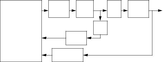
The example system in Figure 32.2 is to control a cart with a hanging pendulum. The cart is driven by a motor. The motor has an attached encoder to measure the motor position. As the cart moves the mass underneath may sway. The position of the hanging mass is measured with a potentiometer.

68HC11	PWM		H-bridge	Vs Motor	ω	cart	x	hanging	θ	mass
68HC11	PWM							mass
								mass
		quadrature			1
		quadrature			---
Digital in		input			D
Digital in				encoder
motor position				encoder	θ
motor position					θ	motor
Analog in		Vθ	potentiometer
Analog in			potentiometer
mass angle

Figure 32.2 System Architecture

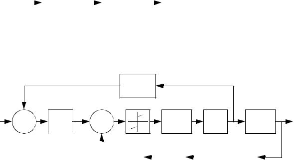
A block diagram for the system is shown in Figure 32.3. A motion generator is used to generate a smooth path for the mass. There are two feedback control loops. The first loop adjusts the motor for general positioning of the system. The inner loop adjusts the output to reduce sway of the cart. The two control signals are added to produce a command signal the drives the load to the final position and then reduces vibrations.

writing guide - 32.11

Cp	generate	update	Cd
	setpoint	setpoints
	setpoint	setpoints
	table

where,

Cp = commanded position

Cd = desired position setpoint

			Cp		encoder
					Kenc
Cd	-	Cpe		Cpc	Cc	Vs	θ p	θ
Cd		Cpe		Cpc	Cc	Vs	θ p	θ	L
			K		PWM		motor	cart and
			K	pp	PWM		motor	mass
				pp				mass

+	+

CLc

Ksp

A/D

potentiometer

Kpot

θ L

– Vzero

where,

Cpe

the position error

Kpp

the proportional gain for position control

the position count from the encoder

the rotational position of the motor

Cpc

output command for position control

the combined motor control output

effective voltage to the motor

position of the motor (cart)

angle of the load from vertical

voltage proportional to angle of load

integer value for load angle

CLc

= output command for sway control

Figure 32.3 System Block Diagram

- for a stationary cart

writing guide - 32.12

··

θ L

··

Mpg sin θ

θ L

··

LMp

where,

mass of cart

x cos θ

= mass of payload

force in suspension arm

Fw =

force from wheels

angle of payload from vertical

length of suspension arm

rw =

radius of cart wheel

··

∑F = – Mpg sin θ L – Mplθ L

– x cos θ LMp

= 0

··

θ L

lθ L

= –g sin θ L – x cos

· 2

··

LMp

∑F = Fp – Mpg cos θ L – θ L

Mpl + x sin θ

= 0

Mpg cos θ

L + θ

· 2

··

Mpl – x sin θ LMp

··

∑Fx = – Mcx + Fp sin θ

L + Fw

= 0

··

L + Fw

= 0

– Mcx + Fp sin θ

··

LMp) sinθ

– Mcx + ( Mpg cos θ L

θ L

Mpl – x sin θ

Mplθ··L

θ·L2Mpl

Mpg cos θ L

··θ

xsin LMp

(1)

L + Fw = 0	(2)

Figure 32.4 FBDs for the suspended mass and the compensator

writing guide - 32.13

Fwrw

ω w + ω

------

= Vs

-----

–

------------

Fw = Vs

– ω

--------

----

--------

rwR

given

= θ wrw

··

Fw = Vs

--------

– x

rwR

(1) --->

rwR

··

· 2

··

– Mcx + ( Mpg cos θ L + θ

L Mpl – x sin θ

LMp) sinθ

L + Vs

--------

– x

----

--------

= 0

– x

rwR

··

· 2

· K2

----

+ ( sin θ

Mp + cos θ

L sin θ

LMpg + θ L ( Mpl sin θ

L) + Vs

--------

– x

--------

= 0

– x Mc + 2

rwR

) 2M

rwR

··

+ J + ( sin θ

--------------------------------------------------------------

= ( cos θ L sin θ L) Mpg + θ L

( Mpl sin θ

L) + Vs

--------

– x

--------

rwR

··

( cos θ

sin θ

)

Mpgrw2

+ θ

Mpl sin θ

Lrw2

x =

--------------------------------------------------------------

+ J + ( sin θ

) 2M

+ J + ( sin θ

) 2M

Krw

–K2

+ x

-----------------------------------------------------------------------

s R( M

+ J + ( sin θ

) 2M

r2 )

R( M

r2 + J + ( sin θ ) 2M

r2 )

Figure 32.5 Adding the differential equation for the motor

writing guide - 32.14

State Equations:

= v

–K2

( cos θ

sin θ

Mpgrw2

= v

)

R-----------------------------------------------------------------------( M

+ J + ( sin θ ) 2M

r2 )

--------------------------------------------------------------

r2 + J + ( sin θ

) 2M

+ ω

Mpl sin θ

Lrw2

Krw

+ V

L M--------------------------------------------------------------

r2 + J + ( sin θ

-----------------------------------------------------------------------

)

s R( M

+ J + ( sin θ )

r2 )

θ·L

ω L

–g

θ L

v cos θ

----- sin

– -----------------

Figure 32.6 State equations for the system

A Scilab program that simulates the given system is given in Figure 32.7.

writing guide - 32.15

//contest.sce

//System component values l = 0.4; // 40cm

Mp = 1.0; // 1kg Mc = 0.2; // 200g

g = 9.81; // good old gravity rw = 0.03; // 6cm dia tires

K = 0.5; // motor speed constant R = 7; // motor resistance

J = 0.005; // rotor inertia

//System state

x0 = 0; // initial conditions for position

v0 = 0;

theta0 = 0.0;// the initial position for the load omega0 = 0.0;

X=[x0, v0, theta0, omega0];

// The controller definition PI = 3.14159;

ppr = 16;// encoder pulses per revolution; Kpot = 1.72;// the angle voltage ratio

Vzero = 2.5;// the voltage when the pendulum is vertical

Vadmax = 5;// the A/D voltage range

Vadmin = 0;

Cadmax = 255;// the A/D converter output limits

Cadmin = 0;

tolerance = 0.5;// the tolerance for the system to settle Kpp = 20;// position feedback gain

Ksp = 2;// sway feedback gain

Vpwmmax = 12; // PWM output limitations in V

Cpwmmax = 255; // PWM input range

Cdeadpos = 100;// deadband limits

Cdeadneg = 95;

function foo=control(Cdesired)

Cp = ppr * X($, 1)/(2*PI*rw);

Cpe = Cdesired - Cp;

Cpc = Kpp * Cpe;

VL = Kpot * X($,3) + 2.5; // assume the zero angle is 2.5V

CL = ((VL - Vadmin) / (Vadmax - Vadmin)) * (Cadmax - Cadmin);

if CL > Cadmax then CL = Cadmax; end// check for voltages over limits if CL < Cadmin then CL = Cadmin; end

CLc = Ksp * (CL - (Cadmax + Cadmin) / 2);

Cc = Cpc + CLc;

Cpwm = 0;

if Cc > 0.5 then// deadband compensation

Cpwm = Cdeadpos + (Cc/Cpwmmax)*(Cpwmmax - Cdeadpos);

end

if Cc <= -0.5 then

Cpwm = -Cdeadneg + (Cc/Cpwmmax)*(Cpwmmax - Cdeadneg);

end

foo = Vpwmmax * (Cpwm / Cpwmmax) ; // PWM output

if foo > Vpwmmax then foo = Vpwmmax; end // clip voltage if too large if foo < -Vpwmmax then foo = -Vpwmmax; end

endfunction

Figure 32.7 A Scilab program to simulate the swaying mass on the crane

writing guide - 32.16

// The motion profile generator

function foo=motion(t_start, t_end, t_now, C_start, C_end) if t_now < t_start then

foo = C_start; elseif t_now > t_end then

foo = C_end;

else

foo = C_start + (C_end - C_start) * (t_now - t_start ) / (t_end - t_start);

end endfunction

// define the state matrix function

term1 = Mc*rw^2 + J;// Precalculate these terms to save time term2 = R*term1;

Xd = 10;// the setpoint 10 turns == 160 pulses

Cd = ppr * Xd / (2 * PI * rw) ;

function foo=derivative(state,t, h) Vs=control(motion(0, 6, t($, 1), 0, Cd));

//Vs=control(Cd);

term3 = cos(state($,3));// precalculate some repeated terms to save time term4 = sin(state($,3));

term5 = term1 + Mp * (term4 * rw)^2;

//printf("%f %f \n", Cd, Vs);

v_dot = -state($,2)*(K^2) / (term5 * R) ...// d/dt v

+term3*term4*Mp*g*rw^2 / term5 ...

+state($,4)^2 * Mp*l*term4*rw^2 / term5 ...

+Vs*K*rw / term5;

foo = [ state($,2), ...// d/dt x = v

v_dot, ...

state($, 4), ...// d/dt theta

-g * term4 / l - state($, 2) * term3 / l ...// d/dt omega ];

endfunction

// Integration Set the time length and step size for the integration steps = 5000;// The number of steps to use

t_start = 0;// the start time - normally use zero t_end = 10;// the end time

h = (t_end - t_start) / steps;// the step size t = [t_start];// an array to store time values for i=1:steps,

t = [t ; t($,:) + h];

X = [X ; X($,:) + h * derivative(X($,:), t($,:), h)];// first order

end

Figure 32.8 A Scilab program to simulate the swaying mass on the crane

writing guide - 32.17

// Graph the values for part e)

plot2d(t, [X(:,1) + l*sin(X(:,3))], [-2], leg="mass position"); //plot2d(t, [X(:,1), 10*X(:, 3)], [-2, -5], leg="position@theta (X 10)"); xtitle('Time (s)');

// printf the values over time intervals = 20;

for time_count=1:intervals,

i = int((time_count - 1)/intervals * steps + 1); xmass = X(i,1) + l*sin(X(i,3));

printf("Mass location at t=%f x=%f \n", i * h, xmass);

// printf("Point at t=%f x=%f, v=%f, theta=%f, omega=%f \n", i * h, X(i, 1), X(i, 2), X(i, 3), X(i, 4));

end

// find the settling time in the results array ts = 0;

for i = 1:steps,

xmass = X(i,1) + l*sin(X(i,3));

if xmass > (Cd + tolerance) then ts = i*h + t_start; end

if xmass < (Cd - tolerance) then ts = i*h + t_start; end

end

printf("\nTheoretical settling time %f \n", ts);

Figure 32.9 A Scilab program to simulate the swaying mass on the crane

<<< < Предыдущая 162 163 164 165 166 167 168 169 170 171 172 173174 / 217174 175 176 177 178 179 180 181 182 183 184 185 186 > Следующая >>>

Соседние файлы в предмете Электротехника

#
23.08.2013338.73 Кб10IrWW_T3_V1p0.pdf
#
23.08.2013334.86 Кб9IrWW_ULTRA_V1p0.pdf
#
23.08.2013453.11 Кб24ISO,IEC 10967-3 standard.Language independent arithmetic.pdf
#
23.08.2013196.61 Кб20ISO8601 standard.Representation of dates and times.pdf
#
23.08.20135.34 Mб261Jack H.Automating manufacturing systems with PLCs.2005.pdf
#
23.08.20135.61 Mб73Jack H.Dynamic system modeling and control.2004.pdf
#
23.08.20133.84 Mб80Jack H.Integration and automation of manufacturing systems.2001.pdf
#
23.08.2013680.22 Кб10Jackson M.A.A system development method.1982.pdf
#
23.08.2013178.08 Кб10Jackson M.JSP in perspective.2001.pdf
#
23.08.2013306.57 Кб13Jain J., Narayan A., Fujita M. - A survey of techniques for formal verification of combinational circuits (1997)(en).pdf
#
23.08.2013255.49 Кб30Jantzen J.Tuning of fuzzy PID controllers.pdf