13.7 Observational errors

All measurements involve certain errors. One might be tempted to believe that, where computers are involved, there would be no error in collecting data, but this is false. Errors are not only a human failing, they occur because of unpredictability in the measurement process, and we have already established throughout this book that computer systems are nothing if not unpredictable. We are thus forced to make estimates of the extent to which our measurements can be in error. This is a difficult matter, but approximate statistical methods are well known in the natural sciences, methods which become increasingly accurate with the amount of data in an experimental sample.

The ability to estimate and treat errors should not be viewed as an excuse for constructing a poor experiment. Errors can only be minimized by design.

13.7.1Random, personal and systematic errors

There are three distinct types of error in the process of observation. The simplest type of error is called random error. Random errors are usually small deviations from the ‘true value’ of a measurement which occur by accident, by unforeseen jitter in the system, or some other influence. By their nature, we are usually ignorant of the cause of random errors, otherwise it might be possible to eliminate them. The important point about random errors is that they are distributed evenly about the mean value of the observation. Indeed, it is usually assumed that they are distributed with an approximately normal or Gaussian profile about the mean. This means that there are as many positive as negative deviations and thus random errors can be averaged out by taking the mean of the observations.

It is tempting to believe that computers would not be susceptible to random errors. After all, computers do not make mistakes. However this is an erroneous belief. The measurer is not the only source of random errors. A better way of expressing this is to say that random errors are a measure of the unpredictability of the measuring process. Computer systems are also unpredictable, since they are constantly influenced by outside agents such as users and network requests.

The second type of error is a personal error. This is an error which a particular experimenter adds to the data unwittingly. There are many instances of this kind of error in the history of science. In a computer-controlled measurement process, this corresponds to any particular bias introduced through the use of specific software, or through the interpretation of the measurements.

The final and most insidious type of error is the systematic error. This is an error which runs throughout all of the data. It is a systematic shift in the true value of the data, in one direction, and thus it cannot be eliminated by averaging. A systematic error leads also to an error in the mean value of the measurement. The sources of systematic error are often difficult to find, since they are often a result of misunderstandings, or of the specific behavior of the measuring apparatus.

In a system with finite resources, the act of measurement itself leads to a change in the value of the quantity one is measuring. In order to measure the CPU usage of a computer system, for instance, we have to start a new program which collects that information, but that program inevitably also uses the CPU and

therefore changes the conditions of the measurement. These issues are well known in the physical sciences and are captured in principles such as Heisenberg’s Uncertainty Principle, Schrodinger’s¨ cat and the use of infinite idealized heat baths in thermodynamics. We can formulate our own verbal expression of this for computer systems:

Principle 67 (Uncertainty). The act of measuring a given quantity in a system with finite resources, always changes the conditions under which the measurement is made, i.e. the act of measurement changes the system.

For instance, in order to measure the pressure in a tyre, you have to let some of the air out, which reduces the pressure slightly. This is not noticeable on a car tyre, but it can be noticeable on a bicycle. The larger the available resources of the system, compared with the resources required to make the measurement, the smaller the effect on the measurement will be.

13.7.2Adding up independent causes

Suppose we want to measure the value of a quantity v whose value has been altered by a series of independent random changes or perturbations v1, v2, . . .

etc. By how much does that series of perturbations alter the value of v? Our first instinct might be to add up the perturbations to get the total:

Actual deviation = v1 + v2 + . . .

This estimate is not useful, however, because we do not usually know the exact values of vi , we can only guess them. In other words, we are working with a set of guesses gi , whose sign we do not know. Moreover, we do not know the signs of the perturbations, so we do not know whether they add or cancel each other out. In short, we are not in a position to know the actual value of the deviation from the true value. Instead, we have to estimate the limits of the possible deviation from the true value v. To do this, we add the perturbations together as though they were independent vectors.

Independent influences are added together using Pythagoras’ theorem, because they are independent vectors. This is easy to understand geometrically. If we think of each change as being independent, then one perturbation v1 cannot affect the value of another perturbation v2. But the only way that it is possible to have two changes which do not have any effect on one another is if they are movements at right angles to one another, i.e. they are orthogonal. Another way of saying this is that the independent changes are like the coordinates x, y, z, . . . of a point which is at a distance from the origin in some set of coordinate axes. The total distance of the point from the origin is, by Pythagoras’ theorem,

d = x2 + y2 + z2 + . . ..

The formula we are looking for, for any number of independent changes, is just the root mean square N -dimensional generalization of this, usually written σ . It is the standard deviation.

13.7.3The mean and standard deviation

In the theory of errors, we use the ideas above to define two quantities for a set of data: the mean and the standard deviation. Now the situation is reversed: we have made a number of observations of values v1, v2, v3, . . . which have a certain scatter, and we are trying to find out the actual value v. Assuming that there are no systematic errors, i.e. assuming that all of the deviations have independent random causes, we define the value v to be the arithmetic mean of the data:

Next we treat the deviations of the actual measurements as our guesses for the error in the measurements:

g1 = v − v1g2 = v − v2

.

.

.

gN = v − vN

and define the standard deviation of the data by

This is clearly a measure of the scatter in the data due to random influences. σ is the root mean square (RMS) of the assumed errors. These definitions are a way of interpreting measurements, from the assumption that one really is measuring the true value, affected by random interference.

An example of the use of standard deviation can be seen in the error bars of the figures in this chapter. Whenever one quotes an average value, the number of data and the standard deviation should also be quoted in order to give meaning to the value. In system administration, one is interested in the average values of any system metric which fluctuates with time.

13.7.4The normal error distribution

It has been stated that ‘Everyone believes in the exponential law of errors; the experimenters because they think it can be proved by mathematics; and the mathematicians because they believe it has been established by observation’ [323]. Some observational data in science satisfy closely the normal law of error, but this is by no means universally true. The main purpose of the normal error law is to provide an adequate idealization of error treatment which is simple to deal with, and which becomes increasingly accurate with the size of the data sample.

The normal distribution was first derived by DeMoivre in 1733, while dealing with problems involving the tossing of coins; the law of errors was deduced

theoretically in 1783 by Laplace. He started with the assumption that the total error in an observation was the sum of a large number of independent deviations, which could be either positive or negative with equal probability, and could therefore be added according to the rule explained in the previous sections. Subsequently Gauss gave a proof of the error law based on the postulate that the most probable value of any number of equally good observations is their arithmetic mean. The distribution is thus sometimes called the Gaussian distribution, or the bell curve.

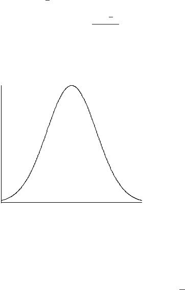
The Gaussian normal distribution is a smooth curve which is used to model the distribution of discrete points distributed around a mean. The probability density function P (x) tells us with what probability we would expect measurements to be distributed about the mean value x (see figure 13.12).

It is based on the idealized limit of an infinite number of points. No experiments have an infinite number of points though, so we need to fit a finite number of points to a normal distribution as best we can. It can be shown that the most probable choice is to take the mean of the finite set to be our estimate of mean

Figure 13.12: The Gaussian normal distribution, or bell curve, peaks at the arithmetic mean. Its width characterizes the standard deviation. It is therefore the generic model for all measurement distributions.

of the ideal set. Of course, if we select at random a sample of N values from the idealized infinite set, it is not clear that they will have the same mean as the full set of data. If the number in the sample N is large, the two will not differ by much, but if N is small, they might. In fact, it can be shown that if we take many random

samples of the ideal set, each of size N , they will have mean values which are

√

themselves normally distributed, with a standard deviation equal to σ/ N. The

quantity

σ

α = √

N

is therefore called the standard error of the mean. This is clearly a measure of the accuracy with which we can claim that our finite sample mean agrees with the actual mean. In quoting a measured value which we believe has a unique or correct value, it is therefore normal to write the mean value, plus or minus the standard error of the mean:

√

Result = x ± σ/ N (for N observations),

where N is the number of measurements. Otherwise, if we believe that the measured value should have a distribution of values, we use the standard deviation as a measure of the error. Many transactional operations in a computer system do not have a fixed value (see next section).

The law of errors is not universally applicable, but it is still almost universally applied, for it serves as a convenient fiction which is mathematically simple.2

13.7.5The Planck distribution

Another distribution which appears in the periodic rhythms of system behavior is the Planck radiation distribution, so named for its origins in the physics of blackbody radiation and quantum theory. This distribution can be derived theoretically as the most likely distribution to arise from an assembly of fluctuations in equilibrium with an indefatigable reservoir or source [54]. The precise reason for its appearance in computer systems is subtle, but has to do with the periodicity imposed by users’ behaviors, as well as the interpretation of transactions as fluctuations. The distribution has the form

λ−m D(λ) = e1/λT − 1 ,

where T is a scale, actually a temperature in the theory of blackbody radiation, and m is a number greater than 2. When m = 3, a single degree of freedom is represented. In ref. [54], Burgess et al. found that a single degree of freedom was sufficient to fit the data measured for a single variable, as one might expect. The shape of the graph is shown in figure 13.13. Figures 13.14 and 13.15 show fits of real data to Planck distributions.

A number of transactions take this form: typically this includes network services that do not stress the performance of a server significantly. Indeed, it was shown in ref. [54] that many transactions on a computing system can be modeled as a linear superposition of a Gaussian distribution and a Planckian distribution, shifted from the origin:

2The applicability of the normal distribution can, in principle, be tested with a χ2 test, but this is seldom used in physical sciences, since the number of observations is usually so small as to make it meaningless.

Figure 13.13: The Planck distribution for several temperatures. This distribution is the shape generated by random fluctuations from a source which is unchanged by the fluctuations. Here, a fluctuation is a computing transaction, a service request or new process.

Figure 13.14: The distribution of system processes averaged over a few daily periods. The dotted line shows the theoretical Planck curve, while the solid line shows actual data. The jaggedness comes from the small amount of data (see next graph). The x-axis shows the deviation about the scaled mean value of 50 and the y-axis shows the number of points measured in class intervals of a half σ . The distribution of values about the mean is a mixture of Gaussian noise and a Planckian blackbody distribution.

by users’ daily rhythms. Other natural periods follow from the largest influences on the system from outside. This must be the case since there are no natural periodic sources internal to the system.3 Apart from the largest sources of perturbation, i.e. the users themselves, there might be other lesser software systems which can generate periodic activity, for instance hourly updates or automated backups. The source might not even be known: for instance, a potential network intruder attempting a stealthy port scan might have programmed a script to test the ports periodically, over a length of time. Analysis of system behavior can sometimes benefit from knowing these periods, e.g. if one is trying to determine a causal relationship between one part of a system and another, it is sometimes possible to observe the signature of a process which is periodic and thus obtain direct evidence for its effect on another part of the system.

Periods in data are in the realm of Fourier analysis. What a Fourier analysis does is to assume that a data set is built up from the superposition of many periodic processes. This might sound like a strange assumption but, in fact, this is always possible. If we draw any curve, we can always represent it as a sum of sinusoidal-waves with different frequencies and amplitudes. This is the complex Fourier theorem:

f (t) = dω f (ω)e−iωt ,

where f (ω) is a series of coefficients. For strictly periodic functions, we can represent this as an infinite sum:

∞

f (t) = cne−2π i nt/T ,

n=0

where T is some time scale over which the function f (t) is measured. What we are interested in determining is the function f (ω), or equivalently the set of coefficients cn which represent the function. These tell us how much of which frequencies are present in the signal f (t), or its spectrum. It is a kind of data prism, or spectral analyzer, like the graphical displays one finds on some music players. In other words, if we feed in a measured sequence of data and Fourier analyze it, the spectral function shows the frequency content of the data which we have measured.

We shall not go into the whys and wherefores of Fourier analysis, since there are standard programs and techniques for determining the series of coefficients. What is more important is to appreciate its utility. If we are looking for periodic behavior in system characteristics, we can use Fourier analysis to find it. If we analyze a signal and find a spectrum such as the one in figure 13.16, then the peaks in the spectrum show the strong periodic content of the signal.

To discover these smaller signals, it will be necessary to remove the louder ones (it is difficult to hear a pin drop when a bomb explodes nearby).

3Of course there is the CPU clock cycle and the revolution of disks, but these occur on a time scale which is smaller than the software operations and so cannot affect system behavior.