Each of the four Fourier Transforms can be subdivided into real and complex versions. The real version is the simplest, using ordinary numbers and algebra for the synthesis and decomposition. For instance, Fig. 8-1 is an example of the real DFT. The complex versions of the four Fourier transforms are immensely more complicated, requiring the use of complex numbers. These are numbers such as: 3 %4 j , where j is equal to &1 (electrical engineers use the variable j, while mathematicians use the variable, i). Complex mathematics can quickly become overwhelming, even to those that specialize in DSP. In fact, a primary goal of this book is to present the fundamentals of DSP without the use of complex math, allowing the material to be understood by a wider range of scientists and engineers. The complex Fourier transforms are the realm of those that specialize in DSP, and are willing to sink to their necks in the swamp of mathematics. If you are so inclined, Chapters 30-33 will take you there.

The mathematical term: transform, is extensively used in Digital Signal Processing, such as: Fourier transform, Laplace transform, Z transform, Hilbert transform, Discrete Cosine transform, etc. Just what is a transform? To answer this question, remember what a function is. A function is an algorithm or procedure that changes one value into another value. For example, y ' 2 x %1 is a function. You pick some value for x, plug it into the equation, and out pops a value for y. Functions can also change several values into a single value, such as: y ' 2 a % 3 b % 4 c , where a, b, and c are changed into y.

Transforms are a direct extension of this, allowing both the input and output to have multiple values. Suppose you have a signal composed of 100 samples. If you devise some equation, algorithm, or procedure for changing these 100 samples into another 100 samples, you have yourself a transform. If you think it is useful enough, you have the perfect right to attach your last name to it and expound its merits to your colleagues. (This works best if you are an eminent 18th century French mathematician). Transforms are not limited to any specific type or number of data. For example, you might have 100 samples of discrete data for the input and 200 samples of discrete data for the output. Likewise, you might have a continuous signal for the input and a continuous signal for the output. Mixed signals are also allowed, discrete in and continuous out, and vice versa. In short, a transform is any fixed procedure that changes one chunk of data into another chunk of data. Let's see how this applies to the topic at hand: the Discrete Fourier transform.

Notation and Format of the Real DFT

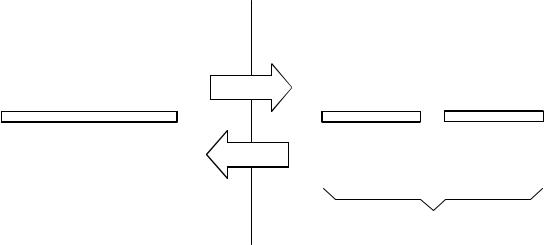
As shown in Fig. 8-3, the discrete Fourier transform changes an N point input signal into two N/2 %1 point output signals. The input signal contains the signal being decomposed, while the two output signals contain the amplitudes of the component sine and cosine waves (scaled in a way we will discuss shortly). The input signal is said to be in the time domain. This is because the most common type of signal entering the DFT is composed of

collectively referred to as X[ ]

FIGURE 8-3

DFT terminology. In the time domain, x[ ] consists of N points running from 0 to N& 1 . In the frequency domain, the DFT produces two signals, the real part, written: Re X [ ], and the imaginary part, written: Im X [ ]. Each of these frequency domain signals are N/2 % 1 points long, and run from 0 to N/2 . The Forward DFT transforms from the time domain to the frequency domain, while the Inverse DFT transforms from the frequency domain to the time domain. (Take note: this figure describes the real DFT. The complex DFT, discussed in Chapter 31, changes N complex points into another set of N complex points).

samples taken at regular intervals of time. Of course, any kind of sampled data can be fed into the DFT, regardless of how it was acquired. When you see the term "time domain" in Fourier analysis, it may actually refer to samples taken over time, or it might be a general reference to any discrete signal that is being decomposed. The term frequency domain is used to describe the amplitudes of the sine and cosine waves (including the special scaling we promised to explain).

The frequency domain contains exactly the same information as the time domain, just in a different form. If you know one domain, you can calculate the other. Given the time domain signal, the process of calculating the frequency domain is called decomposition, analysis, the forward DFT, or simply, the DFT. If you know the frequency domain, calculation of the time domain is called synthesis, or the inverse DFT. Both synthesis and analysis can be represented in equation form and computer algorithms.

The number of samples in the time domain is usually represented by the variable N. While N can be any positive integer, a power of two is usually chosen, i.e., 128, 256, 512, 1024, etc. There are two reasons for this. First, digital data storage uses binary addressing, making powers of two a natural signal length. Second, the most efficient algorithm for calculating the DFT, the Fast Fourier Transform (FFT), usually operates with N that is a power of two. Typically, N is selected between 32 and 4096. In most cases, the samples run from 0 to N&1 , rather than 1 to N.

Standard DSP notation uses lower case letters to represent time domain signals, such as x[ ] , y[ ] , and z[ ] . The corresponding upper case letters are

frequency domain of this signal is called X [ ], and consists of two parts, each an array of N/2 %1 samples. These are called the Real part of X [ ] , written as: Re X [ ], and the Imaginary part of X [ ] , written as: Im X [ ]. The values in Re X [ ] are the amplitudes of the cosine waves, while the values in Im X [ ] are the amplitudes of the sine waves (not worrying about the scaling factors for the moment). Just as the time domain runs from x[0] to x[N&1] , the frequency domain signals run from Re X[0] to Re X[N/2], and from Im X[0] to Im X [N/2]. Study these notations carefully; they are critical to understanding the equations in DSP. Unfortunately, some computer languages don't distinguish between lower and upper case, making the variable names up to the individual programmer. The programs in this book use the array XX[ ] to hold the time domain signal, and the arrays REX[ ] and IMX[ ] to hold the frequency domain signals.

The names real part and imaginary part originate from the complex DFT, where they are used to distinguish between real and imaginary numbers. Nothing so complicated is required for the real DFT. Until you get to Chapter 31, simply think that "real part" means the cosine wave amplitudes, while "imaginary part" means the sine wave amplitudes. Don't let these suggestive names mislead you; everything here uses ordinary numbers.

Likewise, don't be misled by the lengths of the frequency domain signals. It is common in the DSP literature to see statements such as: "The DFT changes an N point time domain signal into an N point frequency domain signal." This is referring to the complex DFT, where each "point" is a complex number (consisting of real and imaginary parts). For now, focus on learning the real DFT, the difficult math will come soon enough.

The Frequency Domain's Independent Variable

Figure 8-4 shows an example DFT with N ' 128 . The time domain signal is contained in the array: x[0] to x[127] . The frequency domain signals are contained in the two arrays: Re X[0] to Re X[64] , and Im X [0] to Im X [64]. Notice that 128 points in the time domain corresponds to 65 points in each of the frequency domain signals, with the frequency indexes running from 0 to 64. That is, N points in the time domain corresponds to N/2 %1 points in the frequency domain (not N/2 points). Forgetting about this extra point is a common bug in DFT programs.

The horizontal axis of the frequency domain can be referred to in four different ways, all of which are common in DSP. In the first method, the horizontal axis is labeled from 0 to 64, corresponding to the 0 to N/2 samples in the arrays. When this labeling is used, the index for the frequency domain is an integer, for example, Re X [k] and Im X [k], where k runs from 0 to N/2 in steps of one. Programmers like this method because it is how they write code, using an index to access array locations. This notation is used in Fig. 8-4b.

In the second method, used in (c), the horizontal axis is labeled as a fraction of the sampling rate. This means that the values along the horizonal axis always run between 0 and 0.5, since discrete data can only contain frequencies between DC and one-half the sampling rate. The index used with this notation is f, for frequency. The real and imaginary parts are written: Re X [f ] and Im X [f ], where f takes on N/2 %1 equally spaced values between 0 and 0.5. To convert from the first notation, k, to the second notation, f , divide the horizontal axis by N. That is, f ' k/N . Most of the graphs in this book use this second method, reinforcing that discrete signals only contain frequencies between 0 and 0.5 of the sampling rate.

The third style is similar to the second, except the horizontal axis is multiplied by 2B. The index used with this labeling is T, a lower case Greek omega. In this notation, the real and imaginary parts are written: Re X [T] and Im X [T], where T takes on N/2 %1 equally spaced values between 0 and B. The parameter, T, is called the natural frequency, and has the units of radians. This is based on the idea that there are 2B radians in a circle. Mathematicians like this method because it makes the equations shorter. For instance, consider how a cosine wave is written in each of