CHAPTER

Properties of Convolution

7

A linear system's characteristics are completely specified by the system's impulse response, as governed by the mathematics of convolution. This is the basis of many signal processing techniques. For example: Digital filters are created by designing an appropriate impulse response. Enemy aircraft are detected with radar by analyzing a measured impulse response. Echo suppression in long distance telephone calls is accomplished by creating an impulse response that counteracts the impulse response of the reverberation. The list goes on and on. This chapter expands on the properties and usage of convolution in several areas. First, several common impulse responses are discussed. Second, methods are presented for dealing with cascade and parallel combinations of linear systems. Third, the technique of correlation is introduced. Fourth, a nasty problem with convolution is examined, the computation time can be unacceptably long using conventional algorithms and computers.

Common Impulse Responses

Delta Function

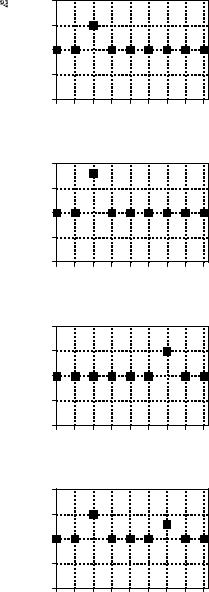
The simplest impulse response is nothing more that a delta function, as shown in Fig. 7-1a. That is, an impulse on the input produces an identical impulse on the output. This means that all signals are passed through the system without change. Convolving any signal with a delta function results in exactly the same signal. Mathematically, this is written:

This property makes the delta function the identity for convolution. This is analogous to zero being the identity for addition ( a % 0 ' a ), and one being the identity for multiplication ( a × 1 ' a ). At first glance, this type of system

123

may seem trivial and uninteresting. Not so! Such systems are the ideal for data storage, communication and measurement. Much of DSP is concerned with passing information through systems without change or degradation.

Figure 7-1b shows a slight modification to the delta function impulse response. If the delta function is made larger or smaller in amplitude, the resulting system is an amplifier or attenuator, respectively. In equation form, amplification results if k is greater than one, and attenuation results if k is less than one:

The impulse response in Fig. 7-1c is a delta function with a shift. This results in a system that introduces an identical shift between the input and output signals. This could be described as a signal delay, or a signal advance, depending on the direction of the shift. Letting the shift be represented by the parameter, s, this can be written as the equation:

Science and engineering are filled with cases where one signal is a shifted version of another. For example, consider a radio signal transmitted from a remote space probe, and the corresponding signal received on the earth. The time it takes the radio wave to propagate over the distance causes a delay between the transmitted and received signals. In biology, the electrical signals in adjacent nerve cells are shifted versions of each other, as determined by the time it takes an action potential to cross the synaptic junction that connects the two.

Figure 7-1d shows an impulse response composed of a delta function plus a shifted and scaled delta function. By superposition, the output of this system is the input signal plus a delayed version of the input signal, i.e., an echo. Echoes are important in many DSP applications. The addition of echoes is a key part in making audio recordings sound natural and pleasant. Radar and sonar analyze echoes to detect aircraft and submarines. Geophysicists use echoes to find oil. Echoes are also very important in telephone networks, because you want to avoid them.

Sample number

FIGURE 7-1

Simple impulse responses using shifted and scaled delta functions.

Calculus-like Operations

Convolution can change discrete signals in ways that resemble integration and differentiation. Since the terms "derivative" and "integral" specifically refer to operations on continuous signals, other names are given to their discrete counterparts. The discrete operation that mimics the first derivative is called the first difference. Likewise, the discrete form of the integral is called the

running sum. It is also common to hear these operations called the discrete derivative and the discrete integral, although mathematicians frown when they hear these informal terms used.

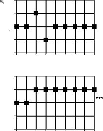
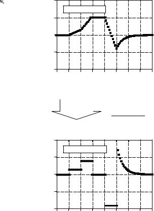
Figure 7-2 shows the impulse responses that implement the first difference and the running sum. Figure 7-3 shows an example using these operations. In 7- 3a, the original signal is composed of several sections with varying slopes. Convolving this signal with the first difference impulse response produces the signal in Fig. 7-3b. Just as with the first derivative, the amplitude of each point in the first difference signal is equal to the slope at the corresponding location in the original signal. The running sum is the inverse operation of the first difference. That is, convolving the signal in (b), with the running sum's impulse response, produces the signal in (a).

These impulse responses are simple enough that a full convolution program is usually not needed to implement them. Rather, think of them in the alternative mode: each sample in the output signal is a sum of weighted samples from the input. For instance, the first difference can be calculated:

That is, each sample in the output signal is equal to the difference between two adjacent samples in the input signal. For instance, y[40] ' x[40] & x[39] . It should be mentioned that this is not the only way to define a discrete derivative. Another common method is to define the slope symmetrically around the point being examined, such as: y[n] ' ( x[n% 1] & x[n& 1] )/ 2 .

2

Sample number

FIGURE 7-2

Impulse responses that mimic calculus operations.

Using this same approach, each sample in the running sum can be calculated by summing all points in the original signal to the left of the sample's location. For instance, if y[n] is the running sum of x[n] , then sample y[40] is found by adding samples x[0] through x[40] . Likewise, sample y[41] is found by adding samples x[0] through x[41] . Of course, it would be very inefficient to calculate the running sum in this manner. For example, if y[40] has already been c a l c u l a t e d , y[41] c a n b e c a l c u l a t e d w i t h o n l y a s i n g l e a d d i t i o n : y[41] ' x[41] % y[40] . In equation form:

Relations of this type are called recursion equations or difference equations. We will revisit them in Chapter 19. For now, the important idea to understand is that these relations are identical to convolution using the impulse responses of Fig. 7-2. Table 7-1 provides computer programs that implement these calculus-like operations.