


136 |
The Scientist and Engineer's Guide to Digital Signal Processing |
|
3.00 |
|
|
a. x[n] |
|
Amplitude |
2.00 |
|
1.00 |
||
|
||
|
0.00 |
-1.00 |
|
|
|
-25 -20 -15 -10 -5 |
0 |
5 |
10 15 20 25 |
Sample number
FIGURE 7-12
Example of convolving a pulse waveform with itself. The Central Limit Theorem shows that a Gaussian waveform is produced when an arbitrary shaped pulse is convolved with itself many times. Figure (a) is an example pulse. In (b), the pulse is convolved with itself once, and begins to appear smooth and regular. In (c), the pulse is convolved with itself three times, and closely approximates a Gaussian.
|
18.0 |
|
|
|
|
|
|
|
|
|
|
|
|
b. x[n] |
x[n] |
|
|
|
|
|
|
|
|
Amplitude |
12.0 |
|
|
|
|
|
|
|
|
|
|
6.0 |
|
|
|
|
|
|
|
|
|
|
|
|
|
|
|
|
|
|
|
|
|
|
|
|
0.0 |
|
|
|
|
|
|
|
|
|
|
|
-6.0 |
|
|
|
|
|
|
|
|
|
|
|
-25 |
-20 |
-15 |
-10 |
-5 |
0 |
5 |
10 |
15 |
20 |
25 |
Sample number
1500
c. x[n]  x[n]
x[n]  x[n]
x[n]  x[n]
x[n]
1000
Amplitude |
500 |
|
0 |
-500
-25 -20 -15 -10 -5 |
0 |
5 |
10 15 20 25 |
Sample number
irregular pulse, purposely chosen to be very unlike a Gaussian. Figure (b) shows the result of convolving this signal with itself one time. Figure (c) shows the result of convolving this signal with itself three times. Even with only three convolutions, the waveform looks very much like a Gaussian. In mathematics jargon, the procedure converges to a Gaussian very quickly. The width of the resulting Gaussian (i.e., F in Eq. 2-7 or 2-8) is equal to the width of the original pulse (expressed as F in Eq. 2-7) multiplied by the square root of the number of convolutions.
Correlation
The concept of correlation can best be presented with an example. Figure 7-13 shows the key elements of a radar system. A specially designed antenna transmits a short burst of radio wave energy in a selected direction. If the propagating wave strikes an object, such as the helicopter in this illustration, a small fraction of the energy is reflected back toward a radio receiver located near the transmitter. The transmitted pulse is a specific shape that we have selected, such as the triangle shown in this example. The received signal will consist of two parts: (1) a shifted and scaled version of the transmitted pulse, and (2) random noise, resulting from interfering radio waves, thermal noise in the electronics, etc. Since radio signals travel at a known rate, the speed of

Chapter 7- Properties of Convolution |
137 |
light, the shift between the transmitted and received pulse is a direct measure of the distance to the object being detected. This is the problem: given a signal of some known shape, what is the best way to determine where (or if) the signal occurs in another signal. Correlation is the answer.
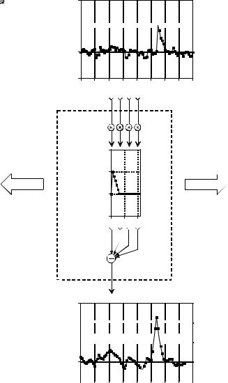
Correlation is a mathematical operation that is very similar to convolution. Just as with convolution, correlation uses two signals to produce a third signal. This third signal is called the cross-correlation of the two input signals. If a signal is correlated with itself, the resulting signal is instead called the autocorrelation. The convolution machine was presented in the last chapter to show how convolution is performed. Figure 7-14 is a similar
FIGURE 7-13
Key elements of a radar system. Like other echo location systems, radar transmits a short pulse of energy that is reflected by objects being examined. This makes the received waveform a shifted version of the transmitted waveform, plus random noise. Detection of a known waveform in a noisy signal is the fundamental problem in echo location. The answer to this problem is correlation.
TRANSMIT RECEIVE
|
200 |
|
|
|
|
|
|
|
|
|
amplitude |
100 |
|
|
|
|
|
|
|
|
|
|
|
|
|
|
|
|
|
|
|
|
Transmitted |
0 |
|
|
|
|
|
|
|
|
|
|
|
|
|
|
|
|
|
|
|
|
|
-100 |
|
|
|
|
|
|
|
|
|
|
-10 |
0 |
10 |
20 |
30 |
40 |
50 |
60 |
70 |
80 |
Sample number (or time)
amplitude |
0.2 |
|
0.1 |
||
|
||
Received |
0 |
|
|
-0.1
-10 |
0 |
10 |
20 |
30 |
40 |
50 |
60 |
70 |
80 |
Sample number (or time)
138 |
The Scientist and Engineer's Guide to Digital Signal Processing |
illustration of a correlation machine. The received signal, x[n] , and the cross-correlation signal, y[n] , are fixed on the page. The waveform we are looking for, t[n] , commonly called the target signal, is contained within the correlation machine. Each sample in y[n] is calculated by moving the correlation machine left or right until it points to the sample being worked on. Next, the indicated samples from the received signal fall into the correlation machine, and are multiplied by the corresponding points in the target signal. The sum of these products then moves into the proper sample in the crosscorrelation signal.
The amplitude of each sample in the cross-correlation signal is a measure of how much the received signal resembles the target signal, at that location. This means that a peak will occur in the cross-correlation signal for every target signal that is present in the received signal. In other words, the value of the cross-correlation is maximized when the target signal is aligned with the same features in the received signal.
What if the target signal contains samples with a negative value? Nothing changes. Imagine that the correlation machine is positioned such that the target signal is perfectly aligned with the matching waveform in the received signal. As samples from the received signal fall into the correlation machine, they are multiplied by their matching samples in the target signal. Neglecting noise, a positive sample will be multiplied by itself, resulting in a positive number. Likewise, a negative sample will be multiplied by itself, also resulting in a positive number. Even if the target signal is completely negative, the peak in the cross-correlation will still be positive.
If there is noise on the received signal, there will also be noise on the crosscorrelation signal. It is an unavoidable fact that random noise looks a certain amount like any target signal you can choose. The noise on the cross-correlation signal is simply measuring this similarity. Except for this noise, the peak generated in the cross-correlation signal is symmetrical between its left and right. This is true even if the target signal isn't symmetrical. In addition, the width of the peak is twice the width of the target signal. Remember, the cross-correlation is trying to detect the target signal, not recreate it. There is no reason to expect that the peak will even look like the target signal.
Correlation is the optimal technique for detecting a known waveform in random noise. That is, the peak is higher above the noise using correlation than can be produced by any other linear system. (To be perfectly correct, it is only optimal for random white noise). Using correlation to detect a known waveform is frequently called matched filtering. More on this in Chapter 17.
The correlation machine and convolution machine are identical, except for one small difference. As discussed in the last chapter, the signal inside of the convolution machine is flipped left-for-right. This means that samples numbers: 1, 2, 3 þ run from the right to the left. In the correlation machine this flip doesn't take place, and the samples run in the normal direction.
Chapter 7- Properties of Convolution |
139 |
2
1 


x[n]
0 |
-1
0 |
10 |
20 |
30 |
40 |
50 |
60 |
70 |
80 |
Sample number (or time)
2 |
|
|
1 |
|
|
t[n] |
|
|
0 |
|
|
-1 |
|
|
0 |
10 |
20 |
3
2 


y[n] 1
1 


0 |
-1 |
|
|
|
|
|
|
|
|
|
|
|
|
|
|
|
|
|
|
|
|
|
|
|
0 |
10 |
20 |
30 |
40 |
50 |
60 |
70 |
80 |
|||
|
|
|
Sample number (or time) |
|
|
|
|||||
FIGURE 7-14
The correlation machine. This is a flowchart showing how the cross-correlation of two signals is calculated. In this example, y [n] is the cross-correlation of x [n] and t [n]. The dashed box is moved left or right so that its output points at the sample being calculated in y [n]. The indicated samples from x [n] are multiplied by the corresponding samples in t [n], and the products added. The correlation machine is identical to the convolution machine (Figs. 6-8 and 6-9), except that the signal inside of the dashed box is not reversed. In this illustration, the only samples calculated in y [n] are where t [n] is fully immersed in x [n].
Since this signal reversal is the only difference between the two operations, it is possible to represent correlation using the same mathematics as convolution. This requires preflipping one of the two signals being correlated, so that the left-for-right flip inherent in convolution is canceled. For instance, when a[n]
a n d b[n] , are convolved to produce c[n] , the equation |
is written: |
a [n ]( b [n ] ' c [n ] . In comparison, the cross-correlation of a[n] |
and b[n] can |