


616 |
The Scientist and Engineer's Guide to Digital Signal Processing |
could be written on the theoretical criteria for this, the practical rules are much simpler. Use as many samples as you think are necessary. After finding the frequency response, go back and repeat the procedure using twice as many samples. If the two frequency responses are adequately similar, you can be assured that the truncation of the impulse response hasn't fooled you in some way.
Cascade and Parallel Stages
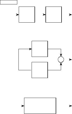
Sophisticated recursive filters are usually designed in stages to simplify the tedious algebra of the z-domain. Figure 33-4 illustrates the two common ways that individual stages can be arranged: cascaded stages and parallel stages with added outputs. For example, a low-pass and high-pass stage can be cascaded to form a band-pass filter. Likewise, a parallel combination of low-pass and high-pass stages can form a band-reject filter. We will call the two stages being combined system 1 and system 2, with their recursion coefficients being called: a0, a1, a2, b1, b2 and A0, A1, A2, B1, B2 , respectively. Our goal is to combine these stages (in cascade or parallel) into a single recursive filter, which we will call system 3, with recursion coefficients given by: a0, a1, a2, a3, a4, b1, b2, b3, b4 .
As you recall from previous chapters, the frequency responses of systems in a cascade are combined by multiplication. Also, the frequency responses of systems in parallel are combined by addition. These same rules are followed by the z-domain transfer functions. This allows recursive systems to be combined by moving the problem into the z-domain, performing the required multiplication or addition, and then returning to the recursion coefficients of the final system.
As an example of this method, we will work out the algebra for combining two biquad stages in a cascade. The transfer function of each stage is found by writing Eq. 33-3 using the appropriate recursion coefficients. The transfer function of the entire system, H [z ] , is then found by multiplying the transfer functions of the two stage:
|
a |
0 |
% a |
|
z & 1 % a |
|
z & 2 |
|
A |
0 |
% A |
|
z & 1 % A |
|
z & 2 |
|||||
H [z ] ' |
|
1 |
|
|
2 |
|
× |
|
1 |
|
|
2 |
|
|||||||
1 & b |
z & 1 |
& b |
2 |
z & 2 |
1 & B |
z & 1 |
& B |
2 |
z & 2 |
|||||||||||
|
|
|||||||||||||||||||
|
|
|
1 |
|
|
|
|
|
|
|
|
1 |
|
|
|
|
|
|||
Multiplying out the polynomials and collecting like terms:
|
a |
A |
0 |
% (a |
A |
% a |
A |
) z & 1 % (a |
A |
% a |
A |
% a |
A |
) z & 2 % (a |
A |
% a |
A |
) z & 3 % (a |
A |
) z & 4 |
||||||||||||
H [z ] ' |
0 |
|
0 |
|
1 |
|
1 |
0 |
|
|
0 |
|
2 |
|
1 |
|
1 |
2 |
0 |
|
|
1 |
2 |
2 |
1 |
|
|
2 |
2 |
|
|
|
|
|
|
1 & (b |
% B |
) z & 1 |
& (b |
% B |
& b |
B |
) z & 2 & (& b |
B |
& b |
B |
) z & 3 & (& b |
B |
) z & 4 |
|
|
||||||||||||||
|
|
|
|
|
|
|||||||||||||||||||||||||||
|
|
|
|
|
1 |
|
1 |
|
|
|
2 |
|
2 |
|
1 |
|
1 |
|
|
|
1 |
2 |
2 |
1 |
|
|
2 |
2 |
|
|
|
|
Chapter 33The z-Transform |
617 |
a. Cascade
FIGURE 33-4
Combining cascade and parallel stages. The z-domain allows recursive stages in a cascade, (a), or in parallel, (b), to be combined into a single system, (c).
|
|
System 1 |
|
System 2 |
||
x[n] |
|
|
y[n] |
|||
|
|
a0, a1, a2 |
|
A0, A1, A2 |
|
|
|
|
|
|
|||
|
|
b1, b2 |
|
B1, B2 |
||
b. Parallel |
|
System 1 |
||||||
|
|
|
a0, a1, a2 |
|||||
x[n] |
b1, b2 |
|||||||
|
|
|
|
y[n] |
||||
|
|
|
|
|
|
|
|
|
|
|
|
|
|
|
|
|
|
System 2
 A0, A1, A2
B1, B2
c. Replacement |
|
|
|
|
x[n] |
System 3 |
|||
a0, a1, a2, a3, a4 |
y[n] |
|||
|
|
|
|
|
|
|
|
||
|
|
b1, b2, b3, b4 |
||
Since this is in the form of Eq. 33-3, we can directly extract the recursion coefficients that implement the cascaded system:
a0 |
' |
a0 A0 |
|
|
a1 ' a0 A1 % a1 A0 |
b1 |
' b1 % B1 |
||
a2 |
' a0 A2 % a1 A1 % a2 A0 |
b2 |
' b2 % B2 & b1 B1 |
|
a3 |
' a1 A2 % a2 A1 |
b3 |
' & b1 B2 & b2 B1 |
|
a4 |
' a2 A2 |
b4 |
' & b2 B2 |
|
The obvious problem with this technique is the large amount of algebra needed to multiply and rearrange the polynomial terms. Fortunately, the entire algorithm can be expressed in a short computer program, shown in Table 33-1. Although the cascade and parallel combinations require different mathematics, they use nearly the same program. In particular, only one line of code is different between the two algorithms, allowing both to be combined into a single program.
618 |
The Scientist and Engineer's Guide to Digital Signal Processing |
|
100 'COMBINING RECURSION COEFFICIENTS OF CASCADE AND PARALLEL STAGES |
||
110 ' |
|
|
120 ' |
'INITIALIZE VARIABLES |
|
130 |
DIM A1[8], B1[8] |
'a and b coefficients for system 1, one of the stages |
140 |
DIM A2[8], B2[8] |
'a and b coefficients for system 2, one of the stages |
150 |
DIM A3[16], B3[16] |
'a and b coefficients for system 3, the combined system |
160 ' |
|
|
170 |
|
'Indicate cascade or parallel combination |
180 |
INPUT "Enter 0 for cascade, 1 for parallel: ", CP% |
|
190 ' |
|
|
200 |
GOSUB XXXX |
'Mythical subroutine to load: A1[ ], B1[ ], A2[ ], B2[ ] |
210 ' |
|
|
220 |
FOR I% = 0 TO 8 |
'Convert the recursion coefficients into transfer functions |
230 |
B2[I%] = -B2[I%] |
|
240 |
B1[I%] = -B1[I%] |
|
250 NEXT I% |
|
|
260 |
B1[0] = 1 |
|
270 |
B2[0] = 1 |
|
280 ' |
|
|
290 |
FOR I% = 0 TO 16 |
'Multiply the polynomials by convolving |
300 |
A3[I%] = 0 |
|
310 |
B3[I%] = 0 |
|
320 |
FOR J% = 0 TO 8 |
|
330 |
IF I%-J% < 0 OR I%-J% > 8 THEN GOTO 370 |
|
340 |
IF CP% = 0 THEN A3[I%] = A3[I%] + A1[J%] * A2[I%-J%] |
|
350 |
IF CP% = 1 THEN A3[I%] = A3[I%] + A1[J%] * B2[I%-J%] + A2[J%] * B1[I%-J%] |
|
360 |
B3[I%] = B3[I%] + B1[J%] * B2[I%-J%] |
|
370 |
NEXT J% |
|
380 NEXT I% |
|
|
390 ' |
|
|
400 |
FOR I% = 0 TO 16 |
'Convert the transfer function into recursion coefficients. |
410 |
B3[I%] = -B3[I%] |
|
420 NEXT I% |
|
|
430 |
B3[0] = 0 |
|
440 ' |
'The recursion coefficients of the combined system now |
|
450 |
END |
'reside in A3[ ] & B3[ ] |
TABLE 33-1
Combining cascade and parallel stages. This program combines the recursion coefficients of stages in cascade or parallel. The recursive coefficients for the two stages being combined enter the program in the arrays: A1[ ], B1[ ], & A2[ ], B2[ ]. The recursion coefficients that implement the entire system leave the program in the arrays: A3[ ], B3[ ].
This program operates by changing the recursive coefficients from each of the individual stages into transfer functions in the form of Eq. 33-3 (lines 220270). After combining these transfer functions in the appropriate manner (lines 290-380), the information is moved back to being recursive coefficients (lines 400 to 430).
The heart of this program is how the transfer function polynomials are represented and combined. For example, the numerator of the first stage being combined is: a0 % a1 z & 1 % a2 z & 2 % a3 z & 3 þ . This polynomial is represented in the program by storing the coefficients: a0, a1, a2, a3 þ , in the array: A1[0], A1[1], A1[2], A1[3]þ . Likewise, the numerator for the second stage is represented by the values stored in: A2[0], A2[1], A2[2], A2[3]þ, and the numerator for the combined system in: A3[0], A3[1], A3[2], A3[3]þ. The
Chapter 33The z-Transform |
619 |
idea is to represent and manipulate polynomials by only referring to their coefficients. The question is, how do we calculate A3[ ], given that A1[ ], A2[ ], and A3[ ] all represent polynomials? The answer is that when two polynomials are multiplied, their coefficients are convolved. In equation form: A1[ ] ( A2[ ] ' A3[ ] . This allows a standard convolution algorithm to find the transfer function of cascaded stages by convolving the two numerator arrays and the two denominator arrays.
The procedure for combining parallel stages is slightly more complicated. In algebra, fractions are added according to:
w |
% |
y |
' |
w@z % y @z |
|
|
x @z |
||
x z |
||||
Since each of the transfer functions is a fraction (one polynomial divided by another polynomial), we combine stages in parallel by multiplying the denominators, and adding the cross products in the numerators. This means that the denominator is calculated in the same way as for cascaded stages, but the numerator calculation is more elaborate. In line 340, the numerators of cascaded stages are convolved to find the numerator of the combined transfer function. In line 350, the numerator of the p a r a l l e l stage combination is calculated as the sum of the two numerators convolved with the two denominators. Line 360 handles the denominator calculation for both cases.
Spectral Inversion
Chapter 14 describes an FIR filter technique called spectral inversion. This is a way of changing the filter kernel such that the frequency response is flipped top-for-bottom. All the passbands are changed into stopbands, and vice versa. For example, a low-pass filter is changed into high-pass, a band-pass filter into band-reject, etc. A similar procedure can be done with recursive filters, although it is far less successful.
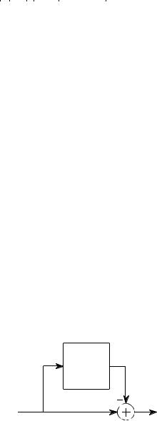
As illustrated in Fig. 33-5, spectral inversion is accomplished by subtracting the output of the system from the original signal. This procedure can be
FIGURE 33-5
Spectral inversion. This procedure is the same as subtracting the output of the system from the original signal.
Original
System
x[n] |
y[n] |

620 |
The Scientist and Engineer's Guide to Digital Signal Processing |
viewed as combining two stages in parallel, where one of the stages happens to be the identity system (the output is identical to the input). Using this approach, it can be shown that the "b" coefficients are left unchanged, and the modified "a" coefficients are given by:
EQUATION 33-6
Spectral inversion. The frequency response of a recursive filter can be flipped top-for- bottom by modifying the "a" coefficients according to these equations. The original coefficients are shown in italics, and the modified coefficients in roman. The "b" coefficients are not changed. This method usually provides poor results.
a0 ' 1 & a0
a1 ' & a1 & b1 a2 ' & a2 & b2 a3 ' & a3 & b3
!
Figure 33-6 shows spectral inversion for two common frequency responses: a low-pass filter, (a), and a notch filter, (c). This results in a high-pass filter, (b), and a band-pass filter, (d), respectively. How do the resulting frequency responses look? The high-pass filter is absolutely terrible! While
Amplitude
Amplitude
2.0
a. Original LP
1.5 


1.0 


0.5 


0.0
0 0.1 0.2 0.3 0.4 0.5
Frequency
2.0
b. Inverted LP
1.5 


1.0 


0.5 


0.0
0 0.1 0.2 0.3 0.4 0.5
Frequency
2.0
c. Original notch
1.5 


Amplitude |
1.0 |
|
|
|
|
|
|
|
|
|
|
|
|
|
0.5 |
|
|
|
|
|
|
0.0 |
|
|
|
|
|
|
0 |
0.1 |
0.2 |
0.3 |
0.4 |
0.5 |
|
|
|
Frequency |
|
|
|
|
2.0 |
|
|
|
|
|
|
|
d. Inverted notch |
|
|
|
|
|
1.5 |
|
|
|
|
|
Amplitude |
|
|
|
|
|
|
Amplitude |
1.0 |
|
|
|
|
|
|
|
|
|
|
|
|
|
0.5 |
|
|
|
|
|
|
0.0 |
|
|
|
|
|
|
0 |
0.1 |
0.2 |
0.3 |
0.4 |
0.5 |
Frequency
FIGURE 33-6
Examples of spectral inversion. Figure (a) shows the frequency response of a 6 pole low-pass Butterworth filter. Figure (b) shows the corresponding high-pass filter obtained by spectral inversion; its a mess! A more successful case is shown in (c) and (d) where a notch filter is transformed in to a band-pass frequency response.