

Young D.C. - Computational chemistry (2001)(en)
.pdf39.2 PERIODIC BOUNDARY CONDITION SIMULATIONS 303
ular dynamics and Monte Carlo methods are discussed in more detail in Chapter 7.
A very important aspect of both these methods is the means to obtain radial distribution functions. Radial distribution functions are the best description of liquid structure at the molecular level. This is because they re¯ect the statistical nature of liquids. Radial distribution functions also provide the interface between these simulations and statistical mechanics.
Another way of predicting liquid properties is using QSPR, as discussed in Chapter 30. QSPR can be used to ®nd a mathematical relationship between the structure of the individual molecules and the behavior of the bulk liquid. This is an empirical technique, which limits the conceptual understanding obtainable. However, it is capable of predicting some properties that are very hard to model otherwise. For example, QSPR has been very successful at predicting the boiling points of liquids.
39.2PERIODIC BOUNDARY CONDITION SIMULATIONS
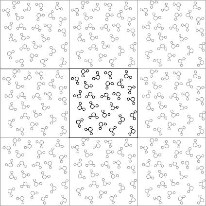
A liquid is simulated by having a number of molecules (perhaps 1000) within a speci®c volume. This volume might be a cube, parallelepiped, or hexagonal cylinder. Even with 1000 molecules, a signi®cant fraction would be against the wall of the box. In order to avoid such severe edge e¨ects, periodic boundary conditions are used to make it appear as though the ¯uid is in®nite. Actually, the molecules at the edge of the next box are a copy of the molecules at the opposite edge of the box, as shown in Figure 39.1.
The use of periodic boundary conditions allows the simulation of a bulk ¯uid, but creates the potential for another type of error. If the longest-range nonbonded forces included in the calculation interact with the same atom in two images of the system, then a long-range symmetry has been unnaturally incorporated into the system. This will result in an additional symmetry in the results, such as a radial distribution function, which is an artifact of the simulation. In order to avoid this problem, the long-range forces are computed only up to a cuto¨ distance that must be less than half of the box's side length. This is called the minimum image convention. It ensures that the system appears to be nonperiodic to any given atom. It also limits the amount of CPU time that will be required for each iteration.
Calculating nonbonded interactions only to a certain distance imparts an error in the calculation. If the cuto¨ radius is fairly large, this error will be very minimal due to the small amount of interaction at long distances. This is why many bulk-liquid simulations incorporate 1000 molecules or more. As the cut- o¨ radius is decreased, the associated error increases. In some simulations, a long-range correction is included in order to compensate for this error.
A radial distribution function can be determined by setting up a histogram for various distances and then looking at all pairs of molecules to construct the diagram. Di¨usion coe½cients can be obtained by measuring the net distances
304 39 SIMULATING LIQUIDS
FIGURE 39.1 Periodic boundary conditions in two dimensions. The molecules that appear to be around the center box are actually copies of the center box.
moved by the solute molecules. Some statistical processes that could be the modeled in a similar way given a more sophisticated setup are chromatographic retention times, crystal growth, and adsorption of molecules on a surface.
These calculations can incorporate various types of constraints. It is most common to run simulations with a ®xed number of atoms and a ®xed volume. In this case, the temperature can be computed from the average kinetic energy of the atoms. It is also possible to adjust the volume to maintain a constant pressure or to scale the velocities to maintain a constant temperature.
If a su½ciently large number of iterations have been performed, the ensemble average of any given property should not change signi®cantly with additional iterations. However, there will be ¯uctuations in any given property computable as a root-mean-square deviation from the ensemble average. These ¯uctuations can be related to thermodynamic derivatives. For example, ¯uctuations in energy can be used to compute a heat capacity for the ¯uid. Alter-
BIBLIOGRAPHY 305
natively, a heat capacity can be determined from its derivative formula after running simulations at two temperatures.
It is also possible to simulate nonequilibrium systems. For example, a bulk liquid can be simulated with periodic boundary conditions that have shifting boundaries. This results in simulating a ¯owing liquid with laminar ¯ow. This makes it possible to compute properties not measurable in a static ¯uid, such as the viscosity. Nonequilibrium simulations give rise to additional technical dif- ®culties. Readers of this book are advised to leave nonequilibrium simulations to researchers specializing in this type of work.
39.3RECOMMENDATIONS
Setting up liquid simulations is more complex than molecular calculations. This is because the issues mentioned in this chapter must be addressed. At least the ®rst time, researchers should plan on devoting a signi®cant amount of work to a liquid simulation project.
BIBLIOGRAPHY
Books dedicated to simulating liquids are
D. M. Hirst, A Computational Approach to Chemistry Blackwell Scienti®c, Oxford (1990).
M. P. Allen, D. J. Tildesley, Computer Simulation of Liquids Oxford, Oxford (1987). C. G. Gray, K. E. Gubbins, Theory of Molecular Fluids Oxford, Oxford (1984).
J. A. Barker, Lattice Theories of the Liquid State Pergamon, New York (1963).
General review articles are
B. Smit, Encycl. Comput. Chem. 3, 1742 (1998).
W. L. Jorgensen, Encycl. Comput. Chem. 4, 2826 (1998).
K. Nakaniski, Chem. Soc. Rev. 22, 177 (1993).
B. J. Alder, E. L. Pollock, Ann. Rev. Phys. Chem. 32, 311 (1981).
Simulating aqueous interfaces is reviewed in
A. Pohorille, Encycl. Comput. Chem. 1, 30 (1998).
Brownian dynamics simulations are reviewed in
J. D. Madura, J. M. Briggs, R. C. Wade, R. R. Gabdoulline, Encycl. Comput. Chem. 1, 141 (1998).
Computing dielectric constants is reviewd in
P. Madden, D. Kivelson, Adv. Chem. Phys. 56, 467 (1984).
306 39 SIMULATING LIQUIDS
Simulation of nonequilibrium processes is reviewed in
P. T. Cummings, A. Baranyai, Encycl. Comput. Chem. 1, 390 (1998).
Describing the structure of liquids is reviewed in
M. S. Wertheim, Ann. Rev. Phys. Chem. 30, 471 (1979). D. Chandler, Ann. Rev. Phys. Chem. 29, 441 (1978).
Simulation of supercritical ¯uids is reviewed in
S. C. Tucker, Encycl. Comput. Chem. 4, 2826 (1998).
A. A. Chialvo, P. T. Cummings, Encycl. Comput. Chem. 4, 2839 (1998).
Computing transport properties is reviewed in
J. H. Dymond, Chem. Soc. Rev. 14, 317 (1985).
Computing viscosity is reviewed in
S. G. Brush, Chem. Rev. 62, 513 (1962).
Computational Chemistry: A Practical Guide for Applying Techniques to Real-World Problems. David C. Young Copyright ( 2001 John Wiley & Sons, Inc.
ISBNs: 0-471-33368-9 (Hardback); 0-471-22065-5 (Electronic)
40 Polymers
Polymers are an extremely important area of study in chemistry. Not only are there many industrial applications, but also the study of them is a complex ®eld of research. Polymers are in the simplest case long-chain molecules with some repeating pattern of functional groups. Most commercially important polymers are organic. The fundamental forces of bonding and intermolecular interactions are the same for polymers as for small molecules. However, many of the polymer properties are dominated by size e¨ects (due to the length of the chain). Thus, simply applying small-molecule modeling techniques is only of limited value.
Polymers are complex systems for a number of reasons. They can be either amorphous or crystalline, or have microscopic domains of both. Most are either amorphous or amorphous with some crystalline domains. Furthermore, this is usually a nonequilibrium state since most production methods do not anneal the material slowly enough to reach an optimal conformation. Thus, the polymer properties vary with the production process (i.e., cooling rate) as well as the molecular structure. The chains of a given polymer may interact primarily by van der Waals forces, hydrogen bonding, p stacking, or chargetransfer interactions. Long-range second-order e¨ects seem to be more important to the description of manmade polymers than is the case for proteins.
This chapter provides the connection between methods described previously and polymer simulation. It does not present the details of many of the polymer simulation methods, which can be found in the references.
40.1LEVEL OF THEORY
One of the simplest ways to model polymers is as a continuum with various properties. These types of calculations are usually done by engineers for determining the stress and strain on an object made of that material. This is usually a numerical ®nite element or ®nite di¨erence calculation, a subject that will not be discussed further in this book.
Polymers are di½cult to model due to the large size of microcrystalline domains and the di½culties of simulating nonequilibrium systems. One approach to handling such systems is the use of mesoscale techniques as described in Chapter 35. This has been a successful approach to predicting the formation and structure of microscopic crystalline and amorphous regions.
307
308 40 POLYMERS
An area of great interest in the polymer chemistry ®eld is structure±activity relationships. In the simplest form, these can be qualitative descriptions, such as the observation that branched polymers are more biodegradable than straightchain polymers. Computational simulations are more often directed toward the quantitative prediction of properties, such as the tensile strength of the bulk material.
One means for performing such predictions are group additivity techniques. They parameterize a table of functional groups and then add the e¨ect of each functional group to obtain polymer properties. Group additivity methods are useful but inherently limited in the accuracy possible. They are generally less reliable when multiple functional groups appear in the repeat unit. However, group additivities are readily calculated on small computers for even the most complex repeat units. More recently, QSPR techniques have become popular (Chapter 30).
Other techniques that work well on small computers are based on the molecules' topology or indices from graph theory. These ®elds of mathematics classify and quantify systems of interconnected points, which correspond well to atoms and bonds between them. Indices can be de®ned to quantify whether the system is linear or has many cyclic groups or cross links. Properties can be empirically ®tted to these indices. Topological and group theory indices are also combined with group additivity techniques or used as QSPR descriptors.
Lattice simulation techniques model a polymer chain by assuming that the possible locations of the atoms fall on the vertices of a regular grid of some sort. This technique has an ability to predict general trends well, but is fairly limited in the absolute accuracy of results. Lattice simulations can use twoor threedimensional lattices, which might be cubic or tetrahedral (diamondlike). The shape of the polymer is simulated by growing the end of the chain with a random-walk algorithm. This means randomly choosing one of the adjacent lattice locations with the exception of doubling back to the previous spot in the chain. Simpler simulations allow the chain to recross itself by crossing the same location twice. Within the accuracy of a lattice model, this is not completely unreasonable since polymers can have twists or knots when there are nonbonded interactions between di¨erent sections of the chain. Some simulations will include an excluded volume e¨ect preventing lattice locations from being used twice.
Another simpli®ed model is the freely jointed or random ¯ight chain model. It assumes all bond and conformation angles can have any value with no energy penalty, and gives a simpli®ed statistical description of elasticity and average end-to-end distance.
The rotational isomeric state (RIS) model assumes that conformational angles can take only certain values. It can be used to generate trial conformations, for which energies can be computed using molecular mechanics. This assumption is physically reasonable while allowing statistical averages to be computed easily. This model is used to derive simple analytic equations that predict polymer properties based on a few values, such as the preferred angle
40.2 SIMULATION CONSTRUCTION |
309 |
between repeat units. The RIS model, with parameters to describe the speci®c polymer of interest, can be used to calculate the following: mean-square end-to- end distance, mean-square radius of gyration, mean-square dipole moment, mean-square optical anisotropy, optical con®guration parameter, molar Kerr constant, and Cotton±Mouton parameter. RIS combined with Monte Carlo sampling techniques can be used to calculate the following: probability distributions for end-to-end lengths and radius of gyration, atom±atom pair correlation function, scattering function, and force±elongation relation for single chains. RIS structures also make a good starting point for MD simulations.
Due to the large size of polymers, most atomic level modeling is by means of molecular mechanics methods. Force ®elds parameterized for general organic systems work well for organic polymers. Because of this, only a few polymer force ®elds have been created, such as PCFF and MSXX. The united-atom approximation (implicit hydrogens) is sometimes used to reduce the computation time. However, all-atom simulations are more sensitive to chain packing and orientational correlations. Fixing bond lengths and angles while maintaining torsional and nonbond interactions improves the simulation time without any apparent loss of accuracy for many properties.
Orbital-based techniques are used for electronic properties, optical properties, and so on. It is usually necessary to make some simplifying assumptions for these calculations. Some semiempirical programs can perform calculations for the one-dimensional in®nite-length chain, which gives a band gap and typical band structure electronic-state information. This assumes that interactions between adjacent polymer strands and the e¨ects of folding are negligible. Another option is to complete simulations on successively larger oligomers and then extrapolate the results to obtain values for the in®nite-length chain. A third option is to examine a typical repeat unit by using the Fock matrix elements from a repeat unit in the middle of a 100to 200-unit oligomer.
40.2SIMULATION CONSTRUCTION
Due to the noncrystalline, nonequilibrium nature of polymers, a statistical mechanical description is rigorously most correct. Thus, simply ®nding a minimum-energy conformation and computing properties is not generally suf- ®cient. It is usually necessary to compute ensemble averages, even of molecular properties. The additional work needed on the part of both the researcher to set up the simulation and the computer to run the simulation must be considered. When possible, it is advisable to use group additivity or analytic estimation methods.
At the beginning of a project, the model system must be determined. Oligomers can be used to model properties that are a function of local regions of the chain only. Simulations of a single polymer strand can be used to determine the tendency to fold in various manners and to ®nd mean end-to-end distances and other properties generally considered the properties of a single mol-
310 40 POLYMERS
ecule. Multiple chains must often be included in a bulk polymer simulation, which is often necessary for modeling the physical properties of the macroscopic material. Periodic boundary conditions are used to simulate the polymer in the bulk system. Liquid-state simulations can also be performed.
The structure of a polymer, which is actually many structures generated by a sampling of conformation space, can be obtained via a number of techniques. Some of the most widely used techniques are as follows:
. Conventional molecular dynamics or Monte Carlo simulations.
.Chain growth algorithms that build up the chain one unit at a time with some randomness in the way units are added. This process can be repeated to yield multiple conformations.
.A reptation algorithm removes units from one end of the chain and adds them to the other end.
.A kink-jump algorithm displaces a few atoms at some point in the chain at each step.
.Conformation search techniques can be used to ®nd very-low-energy conformations, which are most relevant to polymers that will be given a long annealing time.
A number of chain growth techniques have been devised. This means adding units onto an existing structure with some random choice of conformers, excluding any conformers that would result in di¨erent parts of the chain being on top of one another. This sort of model can be implemented using points on a grid with a very simple potential function or using energetics from molecular mechanics calculations. Taking into consideration the energy of various possible ways of adding the monomers will help identify when there is a tendency to develop helical domains, and so on.
Ab initio calculations of polymer properties are either simulations of oligomers or band-structure calculations. Properties often computed with ab initio methods are conformational energies, polarizability, hyperpolarizability, optical properties, dielectric properties, and charge distributions. Ab initio calculations are also used as a spot check to verify the accuracy of molecular mechanics methods for the polymer of interest. Such calculations are used to parameterize molecular mechanics force ®elds when existing methods are insu½cient, which does not happen too often.
40.3PROPERTIES
The property to be predicted must be considered when choosing the method for simulating a polymer. Properties can be broadly assigned into one of two categories: material properties, primarily a function of the nature of the polymer chain itself, or specimen properties, primarily due to the size, shape, and phase
40.3 PROPERTIES 311
of the ®nished object. Thus, material properties are controlled by the choice of monomers, whereas specimen properties are controlled by the manufacturing process. This chapter will focus mostly on material properties, although the mesoscale method does have some ability to predict specimen properties.
Material properties can be further classi®ed into fundamental properties and derived properties. Fundamental properties are a direct consequence of the molecular structure, such as van der Waals volume, cohesive energy, and heat capacity. Derived properties are not readily identi®ed with a certain aspect of molecular structure. Glass transition temperature, density, solubility, and bulk modulus would be considered derived properties. The way in which fundamental properties are obtained from a simulation is often readily apparent. The way in which derived properties are computed is often an empirically determined combination of fundamental properties. Such empirical methods can give more erratic results, reliable for one class of compounds but not for another.
Once a polymer geometry has been described, it can be used to predict density, porosity, and so forth. Geometry alone is often of only minor interest. The purpose of computational modeling is often to determine whether properties of the material justify a synthesis e¨ort. Some of the properties that can be predicted are discussed in the following sections.
Many simulations attempt to determine what motion of the polymer is possible. This can be done by modeling displacements of sections of the chain, Monte Carlo simulations, or reptation (a snakelike motion of the polymer chain as it threads past other chains). These motion studies ultimately attempt to determine a correlation between the molecular motion possible and the macroscopic ¯exibility, hardness, and so on.
The following sections discuss the prediction of a selection of polymer properties. This listing is by no means comprehensive. The sources listed at the end of this chapter provide a much more thorough treatment.
40.3.1Crystallinity
Polymers can be crystalline, but may not be easy to crystallize. Computational studies can be used to predict whether a polymer is likely to crystallize readily. One reason polymers fail to crystallize is that there may be many conformers with similar energies and thus little thermodynamic driving force toward an ordered conformation. Calculations of possible conformations of a short oligomer can be used to determine the di¨erence in energy between the most stable conformer and other low-energy conformers.
In order to reach a crystalline state, polymers must have su½cient freedom of motion. Polymer crystals nearly always consist of many strands with a parallel packing. Simply putting strands in parallel does not ensure that they will have the freedom of movement necessary to then ®nd the low-energy conformer. The researcher can check this by examining the cross-sectional pro®le of the polymer (viewed end on). If the pro®le is roughly circular, it is likely that the chain will be able to change conformation as necessary.
312 40 POLYMERS
The tests in the two previous paragraphs are often used because they are easy to perform. They are, however, limited due to their neglect of intermolecular interactions. Testing the e¨ect of intermolecular interactions requires much more intensive simulations. These would be simulations of the bulk materials, which include many polymer strands and often periodic boundary conditions. Such a bulk system can then be simulated with molecular dynamics, Monte Carlo, or simulated annealing methods to examine the tendency to form crystalline phases.
40.3.2Flexibility
It is generally recognized that the ¯exibility of a bulk polymer is related to the ¯exibility of the chains. Chain ¯exibility is primarily due to torsional motion (changing conformers). Two aspects of chain ¯exibility are typically examined. One is the barrier involved in determining the lowest-energy conformer from other conformers. The second is the range of conformational motion around the lowest-energy conformation that can be accessed with little or no barrier. There is not yet a clear consensus as to which of these aspects of conformational ¯exibility is most closely related to bulk ¯exibility. Researchers are advised to ®rst examine some representative compounds for which the bulk ¯exibility is known.
40.3.3Elasticity
Elastic polymers have long chains with many conformers of nearly identical energy. In the relaxed state, entropy is the driving force for causing the chains to take on some randomly coiled conformation with a mean-square end-to-end distance that is much less than the length of the chain in the most linear conformation, but little di¨erent in energy. Thus, the elastic restoring force is primarily entropic, although there may be a slight energetic component as well. Prediction of elasticity is based on ®nding a large di¨erence in length and small di¨erence in energy between relaxed and linear conformations. This tends to be a qualitative prediction.
Once a rubberband is stretched beyond its elastic region, it becomes much harder to stretch and soon breaks. At this point, the polymer chains are linear and more energy must be applied to slide chains past one another and break bonds. Thus, determining the energy required to break the material requires a di¨erent type of simulation.
Polymers will be elastic at temperatures that are above the glass-transition temperature and below the liqui®cation temperature. Elasticity is generally improved by the light cross linking of chains. This increases the liqui®cation temperature. It also keeps the material from being permanently deformed when stretched, which is due to chains sliding past one another. Computational techniques can be used to predict the glass-transition and liqui®cation temperatures as described below.