Yang Fluidization, Solids Handling, and Processing

Recirculating and Jetting Fluidized Beds 295

Figure 37. Effect of solids loading on gas mixing among concentric jets—tracer injected via air tube at air tube gas velocity of 31 m/s.

3.3Solids Circulation in Jetting Fluidized Beds

The solids circulation pattern and solids circulation rate are important hydrodynamic characteristics of an operating jetting fluidized bed. They dictate directly the solids mixing and the heat and mass transfer between different regions of the bed.

In many applications, the performance of fluidized beds is frequently controlled by the hydrodynamics phenomena occurring in the beds. Applications such as the fluidized bed combustion and gasification of fossil fuels are the cases in point. In those applications, the rates of fuel devolatilization and fines combustion are of the same order of magnitude as the mixing phenomena in a fluidized bed. The mixing and contacting of the gases and solids very often are the controlling factors in the reactor performance. This is especially true in large commercial fluidized beds where only a limited number of discrete feed points for reactants is allowed due to economic considerations. Unfortunately, solids mixing in a fluidized bed has not been studied extensively, especially in large commercial fluidized beds, because of experimental difficulties.

296 Fluidization, Solids Handling, and Processing

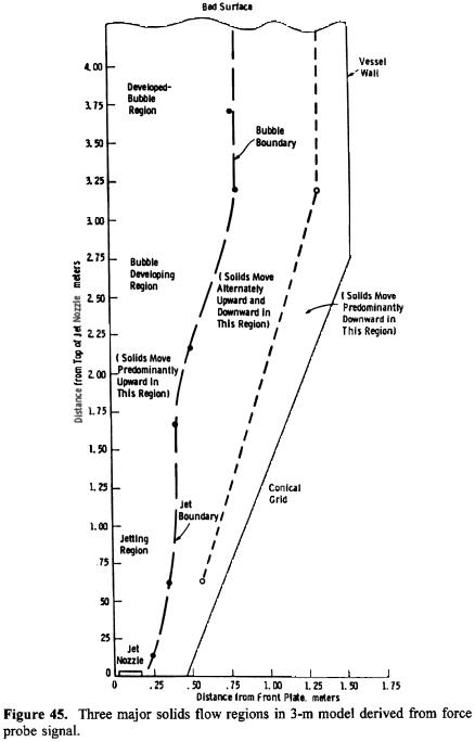
Solids Circulation Pattern. Yang et al. (1986) have shown that, based on the traversing force probe responses, three separate axial solids flow patterns can be identified. In the central core of the bed, the solid flow direction is all upward, induced primarily by the action of the jets and the rising bubbles. In the outer regions, close to the vessel walls, the solid flow is all downward. A transition zone, in which the solids move alternately upward and downward, depending on the approach and departure of the large bubbles, was detected in between these two regions.

Solids mixing and circulation rate were studied in a fluidized bed, 3 m diameter and 10 m in height, by pulse injection of tracer particles with characteristics similar to those inside the bed but with sizes larger than those in the bed. By taking solids samples continuously at different bed locations and analyzing by sieving, the rate of particle mixing and circulation can be calculated. Experiments were conducted in two separate bed configurations. One employed a 0.25 m jet nozzle assembly, a deep-bed configuration with a bed height of 5.5 m; a 0.41 m jet nozzle assembly was used in the second configuration. Crushed acrylic particles, -6 mesh and 1,400 μm in weight-mean average size and 1,100 kg/m3 in density, were used as the bed material.

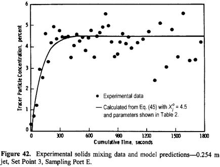
The bed was first operated at the preselected conditions at a steady state; then about 455 kg of the coarse crushed-acrylic particles, similar to that used as the bed material but of sizes larger than 6-mesh, were injected into the bed as fast as possible to serve as the tracer particles. Solids samples were then continuously collected from five different sampling locations at 30-second intervals for the first 18 minutes and at 60-second intervals thereafter. The samples were then sieved and analyzed for coarse tracer particle concentration. Typical tracer particle concentration profiles vs. time at each sampling location are presented in Figs. 38–42 for set point 3.

Typically it took about 160 to 200 seconds to inject a pulse of about 455 kg coarse tracer particles into the bed pneumatically from the coaxial solid feed tube. It can be clearly seen from Figs. 38 to 42 that the tracer particle concentration increases from essentially zero to a final equilibrium value, depending on the location of the sampling port. The steady state was usually reached within about 5 minutes. There is considerable scatter in the data in some cases. This is to be expected because the tracer concentration to be detected is small, on the order of 4%, and absolute uniformity of mixing inside a heterogeneous fluidized bed is difficult to obtain.

Recirculating and Jetting Fluidized Beds 301

Figure 44. Force probe responses for probe penetration from 0.36 m to 0.56 m— 0.13 m from jet nozzle elevation, 46 m/s jet velocity, no solid feed.

In addition to the three solids circulation regions readily identifiable, the approximate jet penetration depth and bubble size can also be obtained from Fig. 45. The jetting region can be taken to be the maximum average value of jet penetration depth. From the jet boundary at the end of the jetting region, an initial bubble diameter can be estimated. This value can be taken to be the minimum value of the initial bubble diameter. The diameter of a fully developed bubble can be obtained from the bubble boundary in the developed-bubble region, as shown in Fig. 45. The central region is thus divided further into three separate regions axially: the jetting region, the bubble-developing region, and the developed–bubble region. Bubbles were observed to coalesce in the bubble–developing region during analysis of the motion pictures taken through the transparent front plate.

304 Fluidization, Solids Handling, and Processing

In the bubble street region

The data do not show any clear dependence on the axial position, z. The axial dependence is thus assumed to be negligible. Equations (37) and (38) are reduced from partial differential equations to ordinary differential equations. If we consider only the annular region, Eq. (38) reduces to

X´J can be approximated by material balance of the coarse particles injected into the bed to serve as the tracer.

Solving for X´J , we have

Substituting Eq. (41) into Eq. (40), and after some mathematical manipulating, we get