348 |
DENSE WAVELENGTH DIVISION MULTIPLEXING |
Suppose that the wavelength is changed from l to l0. Equation (19.4-4) remains valid at another image point (x00; z00). Taking the ratio of the two equations at l and l0 yields
xc |
|
xo |
|
x2 |
1 |
1 |
|
|
|
|
|
|
|
|
|
|
xid xi |
|
þ |
|
þ |
i |
|
|
þ |
|
|
|
|
|
|
|
|
|
|
|
zc |
zo |
2 |
z0 |
zc |
|
|
l |
¼ |
R |
ð |
19 |
4-5 |
Þ |
|
|
|
xo0 |
|
|
|
|
|
|
|
¼ l0 |
xc |
|
|
x2 |
1 |
1 |
|
|
|
: |
|
xid xi |
|
þ |
|
þ |
i |
|
|
þ |
|
|
|
|
|
|
|
|
|
|
zc |
zo0 |
2 |
zo0 |
zc |
|
|
|
|
|
|
|
|
Equating the coefficients of the terms with xi, the new focal point (x00; z00) is obtained as
z00 |
¼ |
|
R |
|
|
|
Rz0 |
|
|
|
|
|
|
|
|
|
1 R |
|
1 |
|
|
|
|
|
zc |
þ |
z0 |
|
|
|
|
|
|
|
|
|
x0 |
|
|
|
|
|
|
|
|
xc |
|
|
|
|
|
ð1 RÞ d |
|
|
|
x0 |
¼ |
z0 |
zc |
|
|
|
|
|
|
|
|
|
0 |
|
|
1 |
|
R 1 |
|
|
|
|
|
|
|
|
|
þ |
|
|
|
|
|
|
|
|
|
|
zc |
|
|
z0 |
|
|
|
where the approximations are based on 1-R 1 and zc z0.
From the above derivation, it is observed that the focal point location z00 is very close to the original z0. Along the x-direction, the dispersion relationship is given as
|
x0 ¼ x00 x0 ¼ z0ð1 RÞ |
x |
|
|
z |
|
xc |
|
|
|
|
|
|
|
0 |
|
|
0 |
|
|
|
|
l |
|
|
l |
d |
zc |
|
|
|
|
|
|
|
|
|
The image points of higher harmonics due to nonlinear encoding with zero-crossings occur when the imaging equation satisfies
|
xc |
|
x00 |
|
xi2 |
1 |
1 |
|
|
xid xi |
|
þ |
|
þ |
|
|
|
þ |
|
¼ nml0 |
ð19:4-10Þ |
zc |
z00 |
2 |
z00 |
zc |
Taking the ratio of Eqs. (19.4-2) and (19.4-10) within the paraxial approximation yields
|
|
|
|
|
|
|
|
|
|
|
|
|
|
|
|
|
|
|
|
|
|
|
|
|
|
xc |
|
|
x0 |
|
|
x2 |
1 |
|
1 |
|
|
|
|
|
|
|
xid xi |
|
|
|
þ |
|
|
þ |
|
i |
|
|
|
|
þ |
|
|
|
|
|
|
|
|
|
zc |
|
z0 |
2 |
z00 |
zc |
|
¼ |
l |
¼ |
R |
ð19:4-11Þ |
|
|
xc |
|
|
x00 |
|
|
|
x2 |
1 |
|
1 |
|
|
ml0 |
m |
xid xi |
|
|
þ |
|
|
þ |
|
i |
|
|
|
|
þ |
|
|
|
|
|
|
|
zc |
|
z00 |
|
2 |
|
z00 |
zc |
|
|
|
|
|
Solving for x00 and z00 in the same way, the higher order harmonic image point
locations are obtained as
z00 |
¼ |
|
|
R |
|
|
|
|
|
|
|
|
|
|
|
|
|
|
|
|
|
|
|
|
|
m R |
þ |
m |
|
|
|
|
|
|
|
|
|
zc |
|
|
z0 |
|
|
|
|
|
|
|
|
|
mx0 |
ðm RÞ d |
xc |
|
|
x0 |
¼ |
|
z0 |
|
zc |
|
|
|
|
|
m |
|
0 |
|
|
|
|
|
m R |
þ |
|
|
|
|
|
|
|
|
|
zc |
z0 |
|
|
|
From the above equations, we observe that a significant move of imaging position in the z-direction occurs as z00 shrinks with increasing harmonic order. This means that the higher harmonics are forced to move towards locations very near the phased array. However, at such close distances to the phased array, the paraxial approximation is not valid. Hence, there is no longer any valid imaging equation. Consequently, the higher harmonics turn into noise. It can be argued that there may still be some imaging equation even if the paraxial approximation is not valid. However, the simulation results discussed in Section 19.4 indicate that there is no such valid imaging equation, and the conclusion that the higher harmonic images turn into noise is believed to be valid. Even if they are imaged very close to the phased array, they would appear as background noise at the relatively distant locations where the image points are. Simulations of Section 19.4 indicate that the signal-to-noise ratio in the presence of such noise is satisfactory, and remains satisfactory as the number of channels are increased.
19.4.1Dispersion Analysis
The analysis in this subsection is based on the simulation results from Eqs. (19.4-6), (19.4-7), (19.4-12), and (19.4-13) in the previous subsection.
Case 1: Spherical wave case (0.1 < zc/z0 < 10)
For the first order harmonics (m ¼ 1), the positions of the desired focal point for l0, that is, x00 and z00 have linear relationship with the wavelength l0. The slope of this relationship decreases as the ratio zc=z0 decreases. For the higher order harmonics ðm 2Þ, x00 is much greater than x0 ¼ 0 and z00 is much less than z0. Therefore, we conclude that the higher order harmonics turn into background noise as discussed in the previous subsection.
Case 2: Plane wave case (zc/z0 1)
In this case, Eqs. (19.4-6), (19.4-7), (19.4-12), and (19.4-13) can be simplified as
z00 |
|
|
|
R |
|
|
R |
1 |
|
|
|
|
|
|
|
|
|
|
|
¼ |
|
|
|
|
|
|
|
|
z0 |
|
|
|
z0 |
|
|
|
|
|
|
|
|
|
m R m |
m |
m |
|
|
|
|
|
|
|
|
|
|
|
|
zc |
|
|
þ |
z0 |
|
|
|
|
|
|
|
|
|
|
|
|
|
|
|
|
|
|
|
|
|
|
|
|
mx0 |
|
|
|
|
|
|
|
|
|
|
|
xc |
|
|
|
|
|
|
|
|
|
|
00 |
¼ |
z0 |
|
|
|
m R m |
|
|
|
|
0 |
|
0 |
m d zc |
x |
|
|
ðm RÞ d |
zc |
|
x |
|
z |
1 |
|
R |
|
xc |
|
|
|
|
|
|
þ |
|
|
|
|
|
|
|
|
|
|
|
|
|
|
|
|
|
|
|
|
|
|
|
|
|
|
|
|
|
|
|
|
|
|
|
|
|
|
|
|
|
|
|
|
zc |
|
z0 |
|
|
|
|
|
|
|
|
|
|
|
|
|
|
|
350 |
DENSE WAVELENGTH DIVISION MULTIPLEXING |
Then, the dispersion relations for the first order (m ¼ 1) are derived as
|
z |
|
|
z |
|
|
|
|
|
|
|
|
|
|
|
|
|
|
|
|
|
|
|
|
|
|
0 |
|
|
|
l |
l |
d zc |
|
l |
l |
|
|
|
|
z0 |
|
xc |
|
|
|
x |
|
|
|
|
|
|
|
|
|
|
|
|
|
|
|
|
|
|
|
19.4.1.1 3-D Dispersion. The mathematical derivation for the 3-D case is very much similar to that for the 2-D case discussed before [Hu, Ersoy]. However, instead of viewing the y variables as constants, thus neglecting them in the derivation, we investigate the y variables along with the x variables, and then obtain independent equations that lead to dispersion relations in both the x-direction and the y-direction. It is concluded that if the x-coordinates and y-coordinates of the points are chosen independently, the dispersion relations are given by
|
x |
|
z |
|
xc |
|
|
|
|
|
|
|
|
|
|
|
0 |
|
|
|
|
|
l |
|
|
l |
dx |
zc |
|
ð19:4-18Þ |
y |
z0 |
|
yc |
|
|
|
|
|
|
|
|
|
|
|
|
|
|
|
|
|
|
|
|
|
l |
|
|
l |
dy |
zc |
|
ð19:4-19Þ |
|
|
|
|
|
|
|
|
|
19.4.2Finite-Sized Apertures
So far in the theoretical discussions, the apertures of the phased array are assumed to be point sources. In general, this assumption works well provided that the phase does not vary much within each aperture. In addition, since the zero-crossings are chosen to be the centers of the apertures, there is maximal tolerance to phase variations, for example, in the range ½ p=2; p=2&. In this section, PHASAR types of devices are considered such that phase modulation is controlled by waveguides truncated at the surface of the phased array.
We use a cylindrical coordinate system (r; f; z) to denote points on an aperture, and a spherical coordinate system (R; ; ) for points outside the aperture. In terms of these variables, the Fresnel–Kirchhoff diffraction formula for radiation fields in the Fraunhofer region is given by [Lu, Ersoy, 1993]
EFFðR; ; Þ ¼ jk 2pR |
þ |
2 |
ðS Eðr; f; 0Þejkr sin cosð fÞrdrdf ð19:4-20Þ |
|
e jkR 1 |
|
cos |
|
|
The transverse electric field of the LP01 mode may be accurately approximated as a Gaussian function:
EGBðr; f; 0Þ ¼ E0e r2=w2 |
ð19:4-21Þ |
where w is the waist radius of the gaussian beam. The field in the Fraunhofer region radiated by such a Gaussian field is obtained by substituting Eq. (19.4-21) into
COMPUTER EXPERIMENTS |
|
|
|
|
|
|
|
|
|
351 |
Eq. (19.4-20). The result is given by |
|
|
|
|
|
|
|
|
|
E |
GBFFð |
R; ; |
Þ ¼ |
jkE |
|
e jkR |
|
w2 |
eðkw sin Þ2=4 |
ð |
19:4-22 |
Þ |
0 |
|
|
|
|
|
R 2 |
|
The far field approximation is valid with the very small sizes of the apertures. Equation (19.4-22) is what is utilized in the simulation of designed phased arrays with finite aperture sizes in Section 19.5.2.
19.5COMPUTER EXPERIMENTS
We first define the parameters used to illustrate the results as follows:
M: the number of phased array apertures (equal to the number of waveguides used in the case of PHASARS)
L: The number of channels (wavelengths to be demultiplexed)
l: The wavelength separation between channels
r: random coefficient in the range of [0,1] defined as the fraction of the uniform spacing length (hence the random shift is in the range ½ r ; r &.
The results are shown in Figures 19.6–19.12. The title of each figure also contains the values of the parameters used. Unless otherwise specified, r is assumed to be 1. In Section 19.5.1, the apertures of the phased array are assumed to be point sources. In Section 19.5.2, the case of finite-sized apertures are considered.
19.5.1Point-Source Apertures
Figure 19.6 shows the intensity distribution on the image plane and the zero-crossing locations of the phased array with 16 channels when the central wavelength is 1550 nm, and the wavelength separation is 0.4 nm between adjacent channels. There are no harmonic images observed on the output plane which is in agreement with the claims of Section 19.3.
In order to verify the dispersion relation given by Eq. (19.4.17), the linear relationship of x with respect to l; d, and different values of z0 were investigated, respectively. The simulation results shown in Figure 19.7 give the slope of each straight line as 1:18; 0:78; 0:40 ð 106Þ, which are in excellent agreement with the theoretically calculated values using Eq. (19.4-17) with d ¼ 30; l0 ¼ 1550 nm, namely, 1.16, 0.77, and 0:39ð 106Þ.
In MISZC, both random sampling and implemention of zero-crossings are crucial to achieve good results. In the following, comparitive results are given to discuss the importance of less than random sampling. Figures 19.8 and 19.9 show the results in cases where total random sampling is not used. All the parameters are the same as in Figure 19.5, except that the parameter r is fixed as 0, 1/4 and 1/2,
352 |
DENSE WAVELENGTH DIVISION MULTIPLEXING |
|
Figure 19.6. |
Output intensity at focal plane (M ¼ 100; L ¼ 16; d ¼ 15; l ¼ 0:4 nm). |
|
|
× 10–3 |
|
|
Output displacement vs wavelength |
|
|
|
|
2.5 |
|
|
|
|
|
|
|
|
|
|
|
2 |
|
|
|
|
|
|
|
|
|
|
(m) |
1.5 |
|
|
|
|
|
|
|
|
|
|
-displacement |
|
|
|
|
|
|
|
|
|
|
1 |
|
|
|
|
|
|
|
|
|
|
X |
|
|
|
|
|
|
|
|
|
|
|
|
0.5 |
|
|
|
|
|
|
|
|
|
|
|
0 |
0.6 |
0.8 |
1 |
1.2 |
1.4 |
1.6 |
1.8 |
2 |
2.2 |
2.4 |
|
0.4 |
|
|
|
|
|
Wavelength (nm) |
|
|
|
|
Figure 19.7. Experimental proof of the linear dispersion relation (M ¼ 100; L ¼ 16; d ¼ 30).
Figure 19.8. Harmonics with nonrandom sampling (M ¼ 100; L ¼ 16; d ¼ 15; l ¼ 0:4 nm; r ¼ 0).
respectively. It is observed that the harmonics of different orders start showing up when r is less than 1, that is, with less than total randomness. In comparison, Figure 19.5 shows the case with r=1, and no harmonics appear since total random sampling is used in this case.
19.5.2Large Number of Channels
The major benefit of the removal of the harmonic images is the ability to increase the possible number of channels. A number of cases with 64, 128, and 256 channels were designed to study large number of channels. In the figure below, the number of
Figure 19.9. Harmonics with partial random sampling (M ¼ 100; L ¼ 16; d ¼ 15; l ¼ 0:4 nm; r ¼ 0:5).
354 |
DENSE WAVELENGTH DIVISION MULTIPLEXING |
Figure 19.10. The case of large number of channels (M ¼ 200; L ¼ 128; l ¼ 0:2 nm).
phased arrayed apertures, the number of channels, and the wavelength separation are represented by M; L, and l, respectively. Figure 19.10 shows the results for M ¼ 200; L ¼ 128, and l ¼ 0:2 nm. The figure consists of two parts. The top figure shows the demultiplexing properties under simultaneous multichannel operation. In this figure, we observe that the nonuniformity among all the channels are in the range of 2 dB. It is also usual in the literature on WDM devices to characterize the cross talk performance by specifying the single channel cross talk figure under the worst case. The bottom figure is the normalized transmission spectrum with respect to the applied wavelengths in the central output port. The
Figure 19.11. The case of Gaussian beam (M ¼ 150; L ¼ 128; d; ¼ 10; l ¼ 0:2 nm).
cross talk value is estimated to be 20 dB. It was observed that cross talk value improves when more apertures (waveguides in the case of PHASARS) are used.
19.5.3Finite-Sized Apertures
The theory for the case of finite-sized apertures yielding beams with Gaussian profile was discussed in Section 19.4.2. Using Eq. (19.4-22), a number of simulations were conducted. The results with 128 channels are shown in Figure 19.11. It is observed that the results are quite acceptable.
19.5.4The Method of Creating the Negative Phase
The experimental results up to this point are for the method of automatic zerocrossings. Figure 19.12 shows an example with the method of creating the negative of the phase of the total phasefront with 16 channels [Hu, Ersoy]. It is observed that the results are equally valid as in the previous cases.
Figure 19.12. Sixteen-channel design with the method of creating the negative phase of the wave front.
356 |
DENSE WAVELENGTH DIVISION MULTIPLEXING |
Figure 19.13. Sixteen-channel design with phase errors (ERR ¼ 0:25p).
19.5.5Error Tolerances
Phase errors are expected to be produced during fabrication. The phase error tolerance was investigated by applying random phase error to each array aperture. The random phase errors were approximated by uniform distribution in the range of [-ERR, ERR] where ERR is the specified maximum error. As long as the maximum error satisfies
the phasors point in similar direction so that there is positive contribution from each aperture. Hence, satisfactory results are expected. This was confirmed by simulation experiments. An example is shown in Figure 19.13, corresponding to ERR ¼ 0:25p.
19.5.63-D Simulations
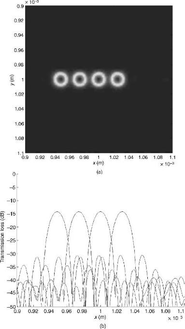
The 3-D method was investigated through simulations in a similar fashion [Hu and Ersoy, 2002]. Figure 19.14 shows one example of focusing and demultiplexing on the image plane (x-y plane at z ¼ z0). The four wavelengths used were 1549.2, 1549.6, 1550, and 1550.4 nm, spaced by 0.4 nm (50 GHz). The array was generated with 50 50 apertures on a 2 2 mm square plane. The diffraction order dx in the x- direction was set to 5, while that in the y-direction, dy, was set to zero.
In Figure 19.14, part (a) shows demultiplexing on the image plane, and part (b) shows the corresponding insertion loss on the output line (x-direction) on the same plane.
It is observed that a reasonably small value of diffraction order (dx 5) is sufficient to generate satisfactory results. This is significant since it indicates that manufacturing in 3-D can indeed be achievable with current technology. A major advantage in 3-D is that the number of apertures can be much larger as compared to 2-D.
Figure 19.14. An example of 3-D design with four wavelengths and exact phase generation.