Ersoy O.K. Diffraction, Fourier optics, and imaging (Wiley, 2006)(ISBN 0471238163)(427s) PEo

effects of these approximations on the reconstructed image depend on several factors, and with proper design, can be minimized [Lohmann, 1970].

The sinc function sinc½cdnðx þ x0Þ& creates a drop-off in intensity in the x- direction proportional to the distance from the center of the image plane. Approximation (a) considers this sinc factor to be nearly constant inside the image region. If the size of the image region is x y, then at the edges x ¼ ð x=2Þ where the effects are most severe, we have sinc½cM c=2&. This implies that a small aperture size c results in less drop-off in intensity. However, this also reduces the brightness of the image. For cM ¼ 1=2, the brightness ratio between the center and the edge of the image region is 9:1. By reducing this product to cM ¼ 1=3, the ratio drops to 2:1. Thus, brightness can be sacrificed for a reduction in intensity drop-off at the edges of the reconstructed image.

The sinc function sincðyWnmdnÞ indicates a drop-off in intensity similar to (a), but in the y-direction. This approximation is a little less dangerous because xdn ¼ 1, which means jyWdnj< 1=2. It is well known that amplitude errors in apertures of coherent imaging systems have little effect on the image because they do not deviate rays like phase errors do [Lohmann, 1970]. To reduce the effects of this approximation, every W could be reduced by a constant factor. However, some brightness would then be sacrificed.

A possible solution to the sinc roll-off in the x direction is to divide the desired image by sinc½cdnðx þ x0Þ&. The desired image f ðx; yÞ becomes

f ðx; yÞ sinc½cdnðx þ x0Þ& :

The same thing cannot be done for the y direction because sincðyWnmdnÞ depends on the aperture parameter Wnm which is yet to be determined. Luckily, this sin c factor is less influential than the x dependent sinc, and design of the hologram can be altered to reduce its effects.

The phase shift exp½2piðxPnmdxÞ& causes a phase error that varies with x location in the image plane. The range of this phase error depends on x and P. Since jxj x=2 ¼ 1=2dn and jPj 1=2M the phase error ranges from zero to p=2M. At its maximum, the phase error corresponds to an optical path length of l=4M. For M ¼ 1, this is within the l=4 Rayleigh criterion for wave aberrations [Lohmann, 1970].

The detrimental effects of these approximations are less when the size of the image region is restricted. The reconstruction errors increase with distance from the center of the image plane. If the reconstruction image region is smaller, the errors are also less.

15.4CONSTANT AMPLITUDE LOHMANN METHOD

The previous section showed that the sinc oscillations due to aperture size is a difficult approximation to deal with. Therefore, it would be desirable, also for the purpose of simpler implementation, to make the height of each aperture constant

cell is quantized. Specifically, there are N possible positions for the center of the aperture (phase), and N=2 þ 1 potential height values (amplitudes) including zero amplitude, since the cell is symmetric in the y direction. A large N produces a pattern close to that of the exact hologram.

For example, we can consider a Lohmann cell divided into 4 4 smaller squares. For a value of c ¼ 1=2 in the Lohmann algorithm, which means that the width of the aperture is fixed at half the width of the entire cell, this cell permits three values of normalized amplitude (0,1/2, and 1) and three values of phase ð p; p=2; 0; and p=2Þ for a total of eight possible combinations. Quantization means there will be error when coding amplitude and phase. Therefore, it makes sense to incorporate an optimization algorithm such as the POCS and to design subholograms iteratively until a convergence condition is met. This topic is further discussed in Section 16.6.

Quantizing aperture positions is useful in practical implementations. For example, spatial light modulators (SLMs) can be used in real time to control amplitude and phase modulation at each hologram point. Unfortunately, the SLM cannot accurately generate an exact Lohmann cell, and quantization is necessary to make realization practical. Similarly, technologies used to make integrated circuits can be used for realizing DOEs as discussed in Sections 11.6 and 11.7. Since precise, continuous surface relief is very difficult, quantization of phase and amplitude is also necessary in all such technologies.

15.6COMPUTER SIMULATIONS WITH THE LOHMANN METHOD

The binary transmission pattern obtained from the Lohmann method can be displayed in one of two ways:

Method 1: To display the exact Lohmann hologram (i.e., aperture size and positions are exactly as specified), the pattern is drawn into a CAD layout, for example using AutoCAD.

Method 2: This is the same as the quantized Lohmann method.

All holograms were designed using parameter values of c ¼ 1=2 and M ¼ 1 [Kuhl, Ersoy]. Setting c ¼ 1=2 means that each aperture has a width equal to half that of the cell. It can also be shown that this value of c maximizes the brightness of the image [Gallagher and Sweeney, 1979]. After choosing c ¼ 1=2, M has to be chosen equal to 1 [Lohmann, 1970]. Also, each approximation discussed in Section 15.3 was assumed to be valid.

Figure 15.3 shows a binary image E of size 64 64, which is placed completely on one side of the image plane.

Because the field in the hologram plane is real, the Fourier transform of the image

Figure 15.4 shows the amplitude of the DFT of the image.

Figure 15.3. The image E used in the generation of the Lohmann hologram.

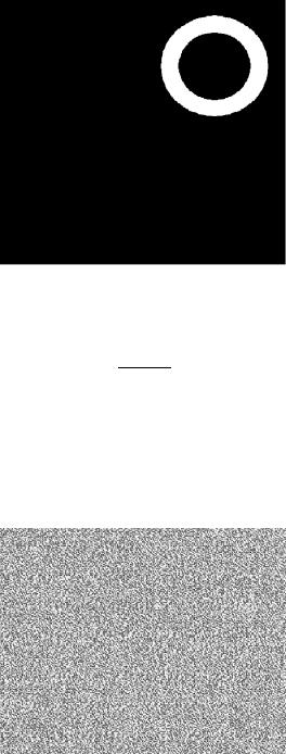
Figure 15.5 shows the Lohmann hologram generated with Method 2 discussed above with 16 levels of quantization.

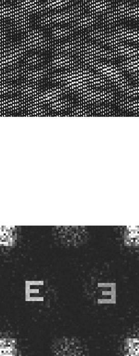
Figure 15.6 shows the simulated reconstruction. The twin images are clearly visible.

The 512 512 gray-scale image shown in Figure 15.8 was also experimented with.

Figure 15.4. The amplitude of the DFT of the image of Figure 15.3.

Figure 15.5. The Lohmann hologram of the image of Figure 15.3.

The computer reconstruction from its Lohmann hologram is shown in Figure 15.8.

The constant amplitude Lohmann method discussed in Section 15.4 was also experimentally investigated with both images, using the iterative optimization approach. The constant amplitude Lohmann hologram for the image E is shown in Figure 15.9. The computer reconstruction obtained from it is shown in Figure 15.10. Similarly, the computer reconstruction obtained from the constant amplitude Lohmann hologram of the gray-level image of Figure 15.8 is shown in Figure 15.11.

Figure 15.6. The computer reconstruction from the hologram of Figure 15.5.

Figure 15.7. The gray-level image of size 512 512.

Comparing Figures 15.6 and 15.10, the desired image E is brighter in the constant amplitude case, but the sharpness of the image E appears to have decreased slightly. The constant amplitude hologram also produced significantly less noise in the corners of the image plane.

Comparing Figures 15.8 and 15.11, the desired image was again brighter and exhibited less noise in the corners of the image plane when compared to the original method.

Figure 15.8. The computer reconstruction obtained from the Lohmann hologram of the gray-level image.

Figure 15.9. The constant amplitude Lohmann hologram of the image of Figure 15.3.

15.7A FOURIER METHOD BASED ON HARD-CLIPPING

It is possible to create a binary Fourier transform DOE by hard-clipping its phase function. In this process, the amplitude information is neglected. For the sake of simplicity, we will explain its analysis in 1-D. Consider a complex function

Aðf Þejfðf Þ

Figure 15.10. The computer reconstruction obtained from the hologram of Figure 15.9.

Figure 15.11. The computer reconstruction obtained from the constant amplitude Lohmann hologram of the gray-level image of Figure 15.8.

modulated with a plane reference wave

ejaf

to generate

Aðf Þejðaf þfðf ÞÞ:

The real part of this signal is passed through the hard-clipping transmission function shown in Figure 15.12.

This function can be modified by adding 0.5 to it so that it changes between 0 and 1. This would have the effect of increasing the DC term of the DFT. The result of hard-clipping the signal with respect to the bipolar transmission function is given by

Figure 15.12. The hard-clipping transmission function.

Figure 15.13. The image used with the hard-clipping method.

hðf Þ can be expressed in terms of its Fourier series representation as [Kozma and Kelly, 1965]

Equation (15.7-2) represents infinitely many images at increasing angles of diffraction. The most important ones are the zero-order image due to 1/2 term and the twin images at angles a due to m ¼ 1 term.

Figure 15.13 shows the image used in experiments with the hard-clipping method. The inverse DFT of this image was coded with the hard-clipping filter. The resulting DOE is shown in Figure 15.14. The forward DFT of the DOE with the

Figure 15.14. The hologram generated with the hard-clipping method.