

Ersoy O.K. Diffraction, Fourier optics, and imaging (Wiley, 2006)(ISBN 0471238163)(427s) PEo
.pdf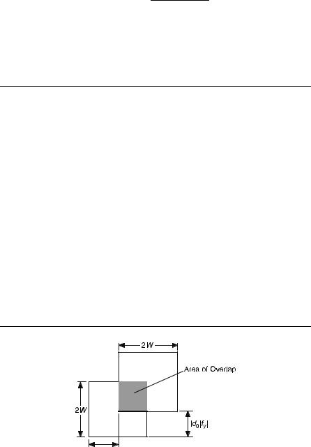
170 |
|
|
|
|
|
|
IMAGING WITH QUASI-MONOCHROMATIC WAVES |
|||||
|
|
|
|
|
|
|
|
|
|
|
|
|
|
|
|
|
|
|
|
|
|
|
|
|
|
|
|
|
|
|
|
|
|
|
|
|
|
|
|
|
|
|
|
|
|
|
|
|
|
|
|
|
|
|
|
|
|
|
|
|
|
|
|
|
|
|
|
|
|
|
|
|
|
|
|
|
|
Figure 10.8. The aperture function for Example 10.9.
EXAMPLE 10.9 An exit aperture function consists of two open squares as shown in Figure 10.8.
Determine
(a)the coherent transfer function
(b)the coherent cutoff frequencies
(c)the amplitude impulse response
(d)the optical transfer function
Solution: (a) The coherent transfer function is the same as the scaled aperture function. Mathematically, the aperture function can be written as
P |
x; y |
|
|
rect |
x 2s |
; |
y |
|
|
rect |
x þ 2s |
; |
y |
|
|
|
|
|||||||||||
Þ ¼ |
|
|
|
|
2s þ |
|
|
2s |
|
|
|
|||||||||||||||||
ð |
|
|
2s |
|
|
|
2s |
|
|
|
||||||||||||||||||
Hð fx; fyÞ is given by |
|
|
|
|
|
|
|
|
|
|
|
|
|
|
|
|
|
|
|
|
|
|
|
|
|
|
|
|
Hð fx; fyÞ ¼ Pðld0 fx; ld0 fyÞ |
|
|
|
|
|
|
|
|
|
|
|
|
|
|
|
|
|
|
||||||||||
|
|
|
l |
d0 fx |
2s d0 fy |
|
|
|
|
|
l |
d0 fx |
|
2s d0 fy |
|
|||||||||||||
¼ rect |
þ |
|
|
; |
l |
|
|
þ rect |
|
|
|
; |
l |
|
||||||||||||||
|
2s |
|
|
|
|
2s |
|
2s |
|
|
2s |
|||||||||||||||||
(b) The cutoff frequencies along the two directions are given by |
|
|
|
|||||||||||||||||||||||||
|
|
|
|
fxc ¼ |
3s |
; |
|
fyc |
¼ |
s |
|
|
|
|
|
|
|
|
|
|
||||||||
|
|
|
|
|
|
|
|
|
|
|
|
|
|
|
|
|
|
|
||||||||||
|
|
|
|
ld0 |
|
ld0 |
|
|
|
|
|
|
|
|
|
|
||||||||||||
(c) The amplitude impulse response hðx; yÞ is the inverse Fourier transform of Hð fx; fyÞ. Let a be equal to ld0s. hðx; yÞ is computed as
hðx; yÞ ¼ |
ðð |
Hð fx; fyÞ ¼ ej2pð fxxþfyyÞdfxdfy |
|
|||||||
|
1 |
|
|
|
|
|
|
|
|
|
|
1 |
|
|
|
|
|
|
|
||
¼ 2 |
3s |
cosð2p fxxÞdfx 2 |
s |
|
|
|||||
ð0 |
ð0 |
cosð2p fyyÞd fy |
||||||||
¼ |
1 sinð6psxÞ sinð2psyÞ |
|
|
|
||||||
p2 |
|
|
x |
|
y |
|
|
|
|
|

COMPUTER COMPUTATION OF THE OPTICAL TRANSFER FUNCTION |
171 |
(d) The total area A under Hð fx; fyÞ equals 8s2. The OTF is given by
ðð1
HI ð fx; fyÞ ¼ Hð fx0; fy0ÞH ð fx0 fx; fy0 fyÞd fx0d fy0
1
A
The computation of the above integral is not trivial and can be best done by the computer.
10.9 COMPUTER COMPUTATION OF THE OPTICAL TRANSFER FUNCTION
The easiest way to compute the discretized OTF is by using the FFT. For this purpose, both hðx; yÞ; Hð fx; fyÞ and HI ð fx; fyÞ, have to be discretized. The discretized coordinates can be written as follows:
x ¼ xn1 |
ð10:9-1Þ |
y ¼ yn2 |
ð10:9-2Þ |
fx ¼ fxk1 |
ð10:9-3Þ |
fy ¼ fyk2 |
ð10:9-4Þ |
hð xn1; yn2Þ, Hð fxk1; fyk2Þ, and HI ð fxk1; fyk2Þ will |
be written as |
hðn1; n2Þ, Hðk1; k2Þ, and HI ðk1; k2Þ, respectively. The size of the matrices involved are assumed to be N1, by N2. In order to use the FFT, the following must be satisfied:
|
|
|
|
x fx ¼ |
1 |
|
|
ð10:9-5Þ |
||||||||
|
|
|
|
|
|
|
||||||||||
|
|
|
N1 |
|||||||||||||
|
|
|
|
y fy ¼ |
1 |
|
|
ð10:9-6Þ |
||||||||
|
|
|
|
|
|
|
||||||||||
|
|
|
N2 |
|||||||||||||
hðn1; n2Þ is approximately given by |
|
|
|
|
|
|
|
|
|
|
|
|
||||
|
hðn1; n2Þ ¼ |
1 |
h0ðn1; n2Þ |
ð10:9-7Þ |
||||||||||||
|
|
|
|
|
||||||||||||
|
K |
|||||||||||||||
where |
|
|
|
|
|
|
|
|
|
|
|
|
|
|
|
|
|
|
N1 |
1 |
|
N2 |
|
1 |
|
|
|
|
|
|
|||
h0ðn1; n2 |
Þ ¼ k1 |
N1 |
k2 |
N2 Hðk1; k2Þej2p N1 þ N2 |
ð10:9-8Þ |
|||||||||||
|
|
X |
|
X |
|
|
|
|
||||||||
|
2 |
|
|
2 |
|
|
|
|
|
|
|
|
n1k1 n2k2 |
|
||
|
¼ |
|
¼ |
|
|
|
|
|
|
|
|
|||||
|
2 |
2 |
|
|
|
|
|
|||||||||
172 |
IMAGING WITH QUASI-MONOCHROMATIC WAVES |
|
and |
|
|
|
K ¼ x yN1N2 |
ð10:9-9Þ |
Hðk1; k2Þ equals Pð ld0 fxk1; ld0 fyk2Þ. N1 and N2 should be chosen such that the pupil function is sufficiently represented. For example, the nonzero portion of the pupil function must be completely covered. In order to minimize the effect of periodicity imposed by the FFT, N1 and N2 should be at least twice as large the minimum values dictated by the nonzero portion of the pupil function.
Once N1 and N2 are properly chosen, Hðk1; k2Þ is arranged as discussed in Section 4.4 so that k1 and k2 satisfy 0 k1 < N1 and 0 k2 < N2 respectively.
HI ðk1; k2Þ is approximately given by
|
|
|
|
|
|
|
|
|
|
x y N1 1 N2 1 |
n1k1 |
n2k2 |
|
|
|
|
|
|||||||||||
|
|
|
|
|
|
|
|
|
|
|
|
|
|
|
|
|
0 jh0ðn1; n2Þj2e j2p |
|
þ |
|
|
|
|
|
||||
|
|
|
|
|
|
|
|
|
|
|
|
|
|
|
|
N1 |
N2 |
|
|
|
||||||||
HI |
ð |
k1 |
; k2 |
Þ ¼ |
|
K2 |
n1 |
¼ |
0 |
n2 |
¼ |
ð |
10:9-10 |
Þ |
||||||||||||||
|
|
|
|
|
|
|
|
|
|
|
|
|
|
|||||||||||||||
|
|
|
|
|
1 |
N1 |
1 N2 1 |
|
|
|
|
|
||||||||||||||||
|
|
|
|
|
|
|
X X |
|
|
|
|
|
|
|
|
|||||||||||||
|
|
|
|
|
|
|
|
|
|
|
|
|
|
|
|
|
X X |
|
|
|
|
|
|
|
|
|||
|
|
|
|
|
|
|
|
|
|
|
|
|
|
|
K |
k1¼0 |
jHðk1; k2Þj2 |
|
|
|
|
|
|
|
|
|||
|
|
|
|
|
|
|
|
|
|
|
|
|
|
|
|
|
k2¼0 |
|
|
|
|
|
|
|
|
|||
or |
|
|
|
|
|
|
|
|
|
|
|
|
0 |
n2 0 jh0ðn1; n2Þj2e j2p |
N1 þ N2 |
|
|
|||||||||||
|
|
|
|
|
|
|
|
|
|
N11N2 |
n1 |
|
|
|||||||||||||||
|
|
|
|
|
|
|
|
|
|
|
N1 |
|
|
1 N2 |
1 |
n1k1 |
n2k2 |
|
|
|
|
|
||||||
HI |
ð |
k1 |
; k2 |
Þ ¼ |
|
|
|
|
¼ |
|
¼ |
|
|
|
|
|
|
ð |
10:9-11 |
Þ |
||||||||
|
|
|
|
|
|
|
N1 1 N2 1 |
|
|
|
|
|||||||||||||||||
|
|
|
|
|
|
X X |
|
|
|
|
|
|
|
|
||||||||||||||
|
|
|
|
|
|
|
|
|
|
|
|
|
|
|
|
X X |
|
|
|
|
|
|
|
|
||||
|
|
|
|
|
|
|
|
|
|
|
|
|
|
|
|
|
|
|
|
jHðk1; k2Þj2 |
|
|
|
|
|
|
|
|
|
|
|
|
|
|
|
|
|
|
|
|
|
|
|
|
k1¼0 |
|
k2¼0 |
|
|
|
|
|
|
|
|
||
The numerator above is the 2-D DFT of jh0ðn1; n2Þj2. HI ðk1; k2Þ above is actually shifted to positive frequencies because of the underlying periodicity. It should be shifted down again to include negative frequencies.
In summary, Hðk1; k2Þ is determined by using the pupil function. h0ðn1; n2Þ is obtained by the inverse DFT of Hðk1; k2Þ according to Eq. (10.9-8). HI ðk1; k2Þ is given by the DFT of jh0ðn1; n2Þj2 normalized by the area under jHðk1; k2Þj2.
Note that fx and fy should be chosen small enough so that h0ðn1; n2Þ is not aliased when computed by using Eq. (10.9-8). Once fx and fy are chosen, N1 and N2 are determined by considering the pupil function as discussed above.
10.9.1Practical Considerations
In studies of the OTF and MTF, ld0 is often chosen to be equal to 1, and the negative signs in the pupil function are neglected so that Hðfx; fyÞ is simply written as Pð fx; fyÞ. Normalization by the area of the pupil function may also be neglected.

ABERRATIONS |
173 |
Another way to generate OTF is by autocorrelating the pupil function with itself.
10.10ABERRATIONS
A diffraction-limited system means the wave of interest is perfect at the exit pupil, and the only imperfection is the finite aperture size. The wave of interest is typically a spherical wave. Aberrations are departures of the ideal wavefront within the exit pupil from its ideal form. They are typically phase errors.
In order to include aberrations, the exit pupil function can be modified as
PAðx; yÞ ¼ Pðx; yÞe jkfAðx;yÞ |
ð10:10-1Þ |
where Pðx; yÞ is the exit pupil function without aberrations, and fAðx; yÞ is the phase error due to aberrations.
The theory of coherent and incoherent imaging developed in the previous sections is still applicable with the replacement of Pðx; yÞ by PAðx; yÞ. For example, the amplitude transfer function becomes
Hðfx; fyÞ ¼ PAð ld0 fx; ld0 fyÞ |
|
|
ð10:10-2Þ |
|||||||||||
|
|
¼ Pð ld0 fx; ld0 fyÞe jkfAð ld0 fx; ld0 fyÞ |
|
|
||||||||||
The optical transfer function can be similarly written as |
|
|
|
|||||||||||
|
|
HI ð fx; fyÞ ¼ |
1 |
|
Að fx; fyÞ |
|
|
|
|
ð10:10-3Þ |
||||
|
|
|
|
|
|
|
||||||||
|
|
|
|
|
ðð Pðld0 fx; ld0 fyÞdfxdfy |
|
|
|
||||||
|
|
|
|
|
1 |
|
|
|
|
|
|
|
|
|
where |
ðð |
PA fx0 þ l 2 ; fy0 þ l |
|
PA fx0 l 2 ; fy0 |
l 2 |
d fx0d fy0 |
||||||||
Að fx; fyÞ ¼ |
2 |
|||||||||||||
|
1 |
|
d0 fx |
|
|
d0 fy |
|
d0 fx |
|
d0 fy |
|
|||
|
|
|
|
|
|
|
|
|||||||
|
1 |
|
|
|
|
|
|
|
|
|
|
|
|
ð10:10-4Þ |
|
|
|
|
|
|
|
|
|
|
|
|
|
|
|
Note that Að fx; fyÞ is to be computed in the area of overlap of the two pupil functions shifted with respect to each other. The ordinary pupil function in this area
equals 1. Letting |
denote integration in the area of overlap, Aðfx; fyÞ can be |
||
written as |
overlap |
|
|
Ð Ð |
|
|
|
|
Að fx; fyÞ ¼overlapðð |
P1P2d fx0d fy0 |
ð10:10-5Þ |

ABERRATIONS |
|
|
|
|
|
|
|
|
|
|
|
|
|
|
|
|
|
|
|
|
|
|
|
|
|
|
|
|
|
|
|
|
|
|
|
|
|
|
|
|
|
|
|
|
|
|
|
|
|
|
|
175 |
Table 10.1. The Zernike polynomials. |
|
|
|
|
|
|
|
|
|
|
|
|
|
|
|
|
|
|
|
|
|
|
|
|
|
|
|
|
|
|
|
|
|
|||||||||||||||||||
|
|
|
|
|
|
|
|
|
|
|
|
|
|
|
|
|
|
|
|
|
|
|
|
|
|
|
|
|
|
|
|
|
|
|
|
|
|
|
|
|
|
|||||||||||
No. |
Polynomial |
|
|
|
|
|
|
|
|
|
|
|
|
|
|
|
|
|
|
|
|
|
|
|
|
|
|
|
|
|
|
|
|
|
|
|
|
|
|
|
|
|||||||||||
|
|
|
|
|
|
|
|
|
|
|
|
|
|
|
|
|
|
|
|
|
|
|
|
|
|
|
|
|
|
|
|
|
|
|
|
|
|
|
|
|
|
|
|
|
|
|
|
|
|
|
|
|
1 |
1 |
|
|
|
|
|
|
|
|
|
|
|
|
|
|
|
|
|
|
|
|
|
|
|
|
|
|
|
|
|
|
|
|
|
|
|
|
|
|
|
|
|
|
|
|
|
|
|
|
|
|
|
2 |
2r cosðyÞ |
|
|
|
|
|
|
|
|
|
|
|
|
|
|
|
|
|
|
|
|
|
|
|
|
|
|
|
|
|
|
|
|
|
|
|
|
|
|
|
|
|
|
|
||||||||
3 |
2r sinðyÞ |
|
|
1 |
|
|
|
|
|
|
|
|
|
|
|
|
|
|
|
|
|
|
|
|
|
|
|
|
|
|
|
|
|
|
|
|
|
|
|
|
|
|
|
|
||||||||
|
|
|
|
r |
|
|
|
|
|
|
|
|
|
|
|
|
|
|
|
|
|
|
|
|
|
|
|
|
|
|
|
|
|
|
|
|
|
|
|
|
|
|
|
|
|
|
|
|
||||
|
p3ð2r2 |
1Þ |
|
|
|
|
|
|
|
|
|
|
|
|
|
|
|
|
|
|
|
|
|
|
|
|
|
|
|
|
|
|
|
|
|
|
|
|
|
|
||||||||||||
|
r |
|
cos 2y |
|
|
|
|
|
|
|
|
|
|
|
|
|
|
|
|
|
|
|
|
|
|
|
|
|
|
|
|
|
|
|
|
|
|
|
|
|
|
|
||||||||||
4 |
p3 |
|
2 |
|
2 |
|
|
|
|
|
|
|
|
|
|
|
|
|
|
|
|
|
|
|
|
|
|
|
|
|
|
|
|
|
|
|
|
|
|
|
|
|
|
|
|
|
|
|
|
|
||
5 |
p6ð |
|
2 |
|
|
|
|
|
Þ |
|
|
|
|
|
|
|
|
|
|
|
|
|
|
|
|
|
|
|
|
|
|
|
|
|
|
|
|
|
|
|
|
|
|
|
|
|
|
|||||
|
r sin 2y |
Þ |
|
|
|
|
|
|
|
|
|
|
|
|
|
|
|
|
|
|
|
|
|
|
|
|
|
|
|
|
|
|
|
|
|
|
|
|
||||||||||||||
|
|
|
|
r |
|
|
ð |
|
|
|
|
|
|
|
|
|
|
|
|
|
|
|
|
|
|
|
|
|
|
|
|
|
|
|
|
|
|
|
|
|
|
|
|
|
|
|
||||||
|
|
|
|
|
|
|
2 r cos y |
|
|
|
|
|
|
|
|
|
|
|
|
|
|
|
|
|
|
|
|
|
|
|
|
|
|
|
|
|
||||||||||||||||
6 |
p6 |
|
|
2 |
|
|
ð |
|
|
Þ |
|
|
|
|
|
|
|
|
|
|
|
|
|
|
|
|
|
|
|
|
|
|
|
|
|
|
|
|
|
|
|
|
|
|
|
|
|
|
||||
|
|
|
|
r |
|
|
|
|
|
|
|
|
|
|
|
|
|
|
|
|
|
|
|
|
|
|
|
|
|
|
|
|
|
|
|
|
|
|
|
|
|
|
|
|
|
|||||||
|
|
|
|
|
|
|
2 r sin y |
|
|
|
|
|
|
|
|
|
|
|
|
|
|
|
|
|
|
|
|
|
|
|
|
|
|
|
|
|
||||||||||||||||
7 |
p8 3 |
|
2 |
|
|
|
|
|
|
|
|
|
|
|
|
|
|
|
|
|
|
|
|
|
|
|
|
|
|
|
|
|
|
|
|
|
|
|
|
|
|
|
|
|
|
|
|
|
||||
8 |
p8ð3 2 |
|
|
|
Þ |
|
|
|
|
|
|
ð Þ |
|
|
|
|
|
|
|
|
|
|
|
|
|
|
|
|
|
|
|
|
|
|
|
|
|
|
|
|||||||||||||
9 |
|
|
|
r |
|
|
|
|
6r |
|
|
|
|
1 |
|
|
|
|
|
|
|
|
|
|
|
|
|
|
|
|
|
|
|
|
|
|
|
|
|
|
|
|
|
|
|
|||||||
p5ð6 |
|
4 |
Þ |
2 |
|
|
|
ð Þ |
|
|
|
|
|
|
|
|
|
|
|
|
|
|
|
|
|
|
|
|
|
|
|
|
|
|
|
|
||||||||||||||||
10 |
r |
|
cos 3y |
|
|
|
|
þ |
|
|
Þ |
|
|
|
|
|
|
|
|
|
|
|
|
|
|
|
|
|
|
|
|
|
|
|
|
|
|
|
|
|
|
|||||||||||
p8ð |
|
3 |
|
|
|
|
|
|
|
|
|
|
|
|
|
|
|
|
|
|
|
|
|
|
|
|
|
|
|
|
|
|
|
|
|
|
|
|
|
|
|
|
|
|
||||||||
|
r sin 3y |
Þ |
|
|
|
|
|
|
|
|
|
|
|
|
|
|
|
|
|
|
|
|
|
|
|
|
|
|
|
|
|
|
|
|
|
|
|
|
||||||||||||||
|
|
|
|
|
|
r |
|
ð |
|
|
|
|
|
|
|
|
|
|
|
|
|
|
|
|
|
|
|
|
|
|
|
|
|
|
|
|
|
|
|
|
|
|
|
|
|
|
|
|||||
|
|
|
|
|
|
|
|
|
|
3 r cos 2y |
|
|
|
|
|
|
|
|
|
|
|
|
|
|
|
|
|
|
|
|
|
|
|
|
|
|||||||||||||||||
11 |
p8 |
|
|
3 |
|
|
ð |
|
|
Þ |
|
|
|
|
|
|
|
|
|
|
|
|
|
|
|
|
|
|
|
|
|
|
|
|
|
|
|
|
|
|
|
|
|
|
|
|
|
|
||||
|
|
|
|
r |
|
|
|
|
|
|
|
|
|
|
|
|
|
|
|
|
|
|
|
|
|
|
|
|
|
|
|
|
|
|
|
|
|
|
|
|
|
|
|
|
||||||||
|
|
|
|
|
|
|
|
3 r sin 2y |
|
|
|
|
|
|
|
|
|
|
|
|
|
|
|
|
|
|
|
|
|
|
|
|
|
|
||||||||||||||||||
12 |
p10 4 |
|
2 |
|
|
|
|
Þ |
|
|
2 |
|
|
|
|
ð |
|
|
Þ |
|
|
|
|
|
|
|
|
|
|
|
|
|
|
|
|
|
|
|
|
|
|
|
||||||||||
|
|
ð |
|
r |
|
|
|
|
|
|
|
|
|
|
|
|
|
|
|
|
|
|
|
|
|
|
|
|
|
|
|
|
|
|
|
|
|
|
|
|||||||||||||
|
|
|
|
|
|
|
|
|
12r |
|
|
|
|
|
3 r cos y |
|
|
|
|
|
|
|
|
|
|
|
|
|
|
|||||||||||||||||||||||
13 |
p10 4 |
|
2 |
|
|
|
|
Þ |
|
|
2 |
|
|
|
ð |
|
|
Þ |
|
|
|
|
|
|
|
|
|
|
|
|
|
|
|
|
|
|
|
|
|
|
|
|
||||||||||
|
|
ð |
|
r |
|
|
|
|
|
|
|
|
|
|
|
|
|
|
|
|
|
|
|
|
|
|
|
|
|
|
|
|
|
|
|
|
|
|
|
|||||||||||||
|
|
|
|
|
|
|
|
|
12r |
|
|
|
|
|
3 r sin y |
|
|
|
|
|
|
|
|
|
|
|
|
|
|
|
||||||||||||||||||||||
14 |
p12 10 |
|
4 |
|
|
|
|
|
|
2 |
|
þ |
|
Þ |
|
|
|
|
|
|
|
|
ð Þ |
|
|
|
|
|
|
|
|
|
|
|
|
|
||||||||||||||||
|
|
ð |
|
r |
|
|
|
|
|
|
|
|
|
|
|
|
|
|
|
|
|
|
|
|
|
|
|
|
|
|
|
|
|
|
|
|
|
|||||||||||||||
|
|
|
|
|
|
|
|
30r |
|
|
|
12r |
|
|
|
|
|
1 |
|
|
|
|
|
|
|
|
|
|
|
|
|
|
|
|
|
|||||||||||||||||
15 |
p12 10 |
|
4 |
|
|
|
|
|
|
2 |
|
þ |
|
Þ |
|
|
|
|
|
|
|
ð Þ |
|
|
|
|
|
|
|
|
|
|
|
|
|
|||||||||||||||||
|
|
|
|
ð |
|
|
|
|
|
|
|
|
|
|
|
|
|
|
|
|
|
|
|
|
|
|
|
|
|
|
|
|
|
|
|
|
|
|
||||||||||||||
|
|
|
r |
|
cos 4y |
|
|
|
|
|
|
|
|
|
|
|
|
|
|
|
|
|
|
|
|
|
|
|
|
|
|
|
|
|
|
|
|
|
|
|
|
|||||||||||
16 |
p7 |
ð |
20 |
|
6 |
|
|
|
|
|
|
|
|
4 |
þ |
|
|
|
|
|
2 |
|
|
|
|
Þ |
|
|
|
|
|
|
|
|
|
|
|
|
|
|
|
|||||||||||
|
|
|
|
|
|
|
|
|
|
|
|
|
|
|
|
|
|
|
|
|
|
|
|
|
|
|
|
|
|
|
|
|
|
|
|
|
|
|
|
|
||||||||||||
|
r |
|
sin 4y |
|
|
|
|
|
|
|
|
|
|
|
|
|
|
|
|
|
|
|
|
|
|
|
|
|
|
|
|
|
|
|
|
|
|
|
|
|
||||||||||||
17 |
p10 |
|
4 |
|
|
|
|
ð |
|
|
|
Þ |
|
|
|
|
|
|
|
|
|
|
|
|
|
|
|
|
|
|
|
|
|
|
|
|
|
|
|
|
|
|
|
|
|
|
|
|||||
|
|
|
|
r |
|
|
|
|
|
|
|
|
|
|
|
|
|
|
|
|
|
|
|
|
|
|
|
|
|
|
|
|
|
|
|
|
|
|
|
|
|
|
|
|
|
|||||||
|
|
|
|
|
|
|
|
4 r cos 3y |
|
|
|
|
|
|
|
|
|
|
|
|
|
|
|
|
|
|
|
|
|
|
|
|
|
|||||||||||||||||||
18 |
p10 |
|
4 |
|
|
|
ð |
|
|
|
Þ |
|
|
|
|
|
|
|
|
|
|
|
|
|
|
|
|
|
|
|
|
|
|
|
|
|
|
|
|
|
|
|
|
|
|
|
||||||
|
|
|
|
r |
|
|
|
|
|
|
|
|
|
|
|
|
|
|
|
|
|
|
|
|
|
|
|
|
|
|
|
|
|
|
|
|
|
|
|
|
|
|
|
|
||||||||
|
|
|
|
|
|
|
|
4 r sin 3y |
|
|
|
|
|
|
|
|
|
|
|
|
|
|
|
|
|
|
|
|
|
|
|
|
|
|
||||||||||||||||||
19 |
p12 5 |
|
2 |
|
|
|
|
Þ |
|
|
3 |
|
|
|
|
ð |
|
|
Þ |
|
|
|
|
|
|
|
|
|
|
|
|
|
|
|
|
|
|
|
|
|
|
|
||||||||||
|
|
ð |
|
r |
|
|
|
|
|
|
|
|
|
|
|
|
|
|
|
|
|
|
|
|
|
|
|
|
|
|
|
|
|
|
|
|
|
|
|
|||||||||||||
|
|
|
|
|
|
|
|
|
20r |
|
|
|
|
|
6 r cos 2y |
|
|
|
|
|
|
|
|
|
|
|
|
|||||||||||||||||||||||||
20 |
p12 5 |
|
2 |
|
|
|
|
Þ |
|
|
3 |
|
|
|
ð |
|
|
Þ |
|
|
|
|
|
|
|
|
|
|
|
|
|
|
|
|
|
|
|
|
|
|
|
|
||||||||||
|
|
ð |
|
r |
|
|
|
|
|
|
|
|
|
|
|
|
|
|
|
|
|
|
|
|
|
|
|
|
|
|
|
|
|
|
|
|
|
|
|
|||||||||||||
|
|
|
|
|
|
|
|
|
20r |
|
|
|
|
|
6 r sin 2y |
|
|
|
|
|
|
|
|
|
|
|
|
|
||||||||||||||||||||||||
21 |
p14 15 |
|
4 |
|
|
|
|
|
|
2 |
|
þ |
|
Þ |
|
|
|
2 |
|
|
|
|
|
|
ð |
|
Þ |
|
|
|
|
|
|
|
|
|
|
|
||||||||||||||
23 |
|
|
|
|
ð |
|
|
|
|
|
|
|
|
|
|
|
|
|
|
|
|
|
|
|
|
|
r |
|
y |
|
|
|
|
|
|
|
|
|
||||||||||||||
4 r |
|
|
|
|
|
|
r |
|
|
|
|
|
|
|
r |
|
|
|
|
|
|
|
|
|
|
|
|
|
|
|
|
|
|
|
|
|
|
|||||||||||||||
22 |
p14 15 |
|
4 |
|
|
|
|
|
|
2 |
|
þ |
|
Þ |
|
|
|
2 |
|
|
|
|
|
ð |
|
|
Þ |
|
|
|
|
|
|
|
|
|
|
|
||||||||||||||
|
|
|
|
|
ð |
|
|
|
|
|
|
|
|
|
|
|
|
|
|
|
|
|
|
|
|
|
|
|
|
|
|
|
|
|
|
|
|
|
|
|
|
|||||||||||
|
ð |
35 |
|
6 |
|
60 |
|
|
4 |
|
þ |
30 |
|
|
2 |
|
4 |
Þ |
|
|
|
cos |
ð Þ |
|
|
|
|
|
|
|
|
|||||||||||||||||||||
|
|
|
|
|
|
|
|
|
|
|
|
|
|
|
|
|
|
|
|
|
|
|
|
|
|
|
|
|
|
|
|
|
||||||||||||||||||||
24 |
4ð35r6 60r4 þ 30r2 4Þr sinðyÞ |
|
|
|
|
|
|
|
|
|||||||||||||||||||||||||||||||||||||||||||
25 |
3ð70r8 140r6 þ 90r4 20r2 þ 1Þ |
|
|
|
|
|
|
|
|
|||||||||||||||||||||||||||||||||||||||||||
27 |
r |
|
sin 5y |
|
|
|
|
|
|
|
|
|
|
|
|
|
|
|
|
|
|
|
|
|
|
|
|
|
|
|
|
|
|
|
|
|
|
|
|
|
||||||||||||
26 |
p12r5 cosð5yÞ |
|
|
|
|
|
|
|
|
|
|
|
|
|
|
|
|
|
|
|
|
|
|
|
|
|
|
|
|
|
|
|
|
|
|
|
||||||||||||||||
28 |
|
|
|
r |
|
|
|
|
|
5 r cos 4y |
|
|
|
|
|
|
|
|
|
|
|
|
|
|
|
|
|
|
|
|
|
|
|
|
|
|||||||||||||||||
|
p12 |
|
5 |
|
|
|
ð |
|
|
|
Þ |
|
|
|
|
|
|
|
|
|
|
|
|
|
|
|
|
|
|
|
|
|
|
|
|
|
|
|
|
|
|
|
|
|
|
|
||||||
29 |
|
|
|
r |
|
|
|
|
|
|
|
|
|
|
|
|
|
|
|
|
|
|
|
|
|
|
|
|
|
|
|
|
|
|
|
|
|
|
|
|
|
|
|
|
||||||||
|
|
|
|
|
|
|
5 r sin 4y |
|
|
|
|
|
|
|
|
|
|
|
|
|
|
|
|
|
|
|
|
|
|
|
|
|
|
|||||||||||||||||||
|
p14 6 |
|
2 |
|
|
|
|
Þ |
|
|
4 |
|
|
|
|
ð |
|
|
Þ |
|
|
|
|
|
|
|
|
|
|
|
|
|
|
|
|
|
|
|
|
|
|
|
||||||||||
30 |
|
|
|
|
ð |
|
|
|
|
|
|
|
|
|
|
|
|
|
|
|
|
|
|
|
|
|
|
|
|
|
|
|
|
|
|
|
|
|
|
|
|
|
|
|||||||||
4 r |
|
|
|
30r |
|
|
|
10 r cos 3y |
|
|
|
|
|
|
|
|
|
|
|
|
|
|
||||||||||||||||||||||||||||||
|
p14 6 |
|
2 |
|
|
|
|
Þ |
|
|
4 |
|
|
|
ð |
|
|
Þ |
|
|
|
|
|
|
|
|
|
|
|
|
|
|
|
|
|
|
|
|
|
|
|
|
||||||||||
|
|
|
|
|
ð |
|
|
|
|
|
|
|
|
|
|
|
|
|
|
|
|
|
|
|
|
|
|
|
|
|
|
|
|
|
|
|
|
|
|
|
|
|
|
|||||||||
|
ð |
21 |
|
4 |
|
|
|
|
|
|
|
2 |
|
þ |
|
|
|
|
Þ |
3 |
|
|
|
|
|
ð |
|
|
|
|
Þ |
|
|
|
|
|
|
|
|
|
|
|
|
|
||||||||
|
|
|
|
|
|
|
|
|
|
|
|
|
|
|
|
|
|
|
|
|
|
|
|
|
|
|
|
|
|
|
|
|
|
|
|
|
|
|
|
|
|
|
||||||||||
31 |
4ð21r4 30r2 þ 10Þr3 sinð3yÞ |
|
|
|
|
|
|
|
|
|
|
|
|
|
||||||||||||||||||||||||||||||||||||||
33 |
ð |
|
r |
|
|
105r |
|
þ 60r |
|
10Þr sinð2yÞ |
|
|
|
|
|
|
||||||||||||||||||||||||||||||||||||
32 |
p18ð56r6 |
|
|
105r4 |
þ 60r2 |
|
10Þr2 cosð2yÞ |
|
|
|
|
|
|
|||||||||||||||||||||||||||||||||||||||
34 |
|
|
|
|
r |
|
|
|
|
|
|
280r |
|
|
|
|
210r |
|
|
|
|
60r |
|
5 r cos y |
|
|
|
|
||||||||||||||||||||||||
35 |
p18 56 |
|
6 |
|
|
|
|
|
|
|
|
|
|
4 |
|
|
|
|
|
|
|
|
2 |
|
|
|
|
|
|
|
|
|
|
2 |
|
5 r sin y |
|
|
|
|
||||||||||||
|
|
|
|
r |
|
|
|
|
|
|
280r |
|
|
|
|
210r |
|
|
|
|
60r |
|
|
|
|
|
||||||||||||||||||||||||||
|
p20 126 |
|
|
8 |
|
|
|
|
|
|
|
6 |
|
þ |
|
|
|
|
|
|
|
|
4 |
|
|
|
|
|
|
2 |
þ |
Þ |
|
ð Þ |
|
|
|
|
||||||||||||||
36 |
|
|
|
|
ð |
|
|
r |
|
|
|
|
|
|
|
|
|
|
|
|
|
|
|
|
|
|
|
|
|
|
|
|
|
|
|
|
|
|
|
|||||||||||||
ð |
|
|
|
|
|
630r |
|
|
þ 560r |
|
|
210r |
þ 30r |
1Þ |
|
|
|
|
||||||||||||||||||||||||||||||||||
|
p20 126 |
|
|
8 |
|
|
|
|
|
|
|
6 |
|
þ |
|
|
|
|
|
|
|
|
4 |
|
|
|
|
|
|
2 |
þ |
Þ |
|
ð Þ |
|
|
|
|
||||||||||||||
37 |
|
ð |
|
|
|
|
r |
|
|
|
|
|
|
|
|
|
|
|
|
|
|
|
|
|
|
|
|
|
|
|
|
|
|
|
|
42r 1 |
||||||||||||||||
|
|
|
|
|
|
|
|
|
|
|
|
2772r |
|
|
|
|
|
3150r 1680r |
|
420r |
|
|
||||||||||||||||||||||||||||||
|
p11 252 |
|
|
10 |
|
|
|
|
|
|
|
8 |
|
|
|
þ |
|
|
|
|
|
6 |
|
|
|
|
|
4 |
|
2 |
|
|
|
|
þ Þ |
|||||||||||||||||
|
p |
|
|
|
|
|
|
12 |
|
|
|
|
|
|
|
|
10 |
|
|
|
|
|
|
|
|
|
8 |
|
6 |
þ |
|
4 |
2 |
|||||||||||||||||||
|
|
13 924 |
|
|
|
|
|
|
|
|
|
|
|
|
|
|
|
|
|
|
|
|
|
|
|
|
|
|
|
|
|
|
|
|
|
|||||||||||||||||
|
|
|
|
|
ð |
|
|
|
|
|
|
|
|
|
|
|
|
|
|
|
|
|
|
|
|
|
|
|
|
|
|
|
|
|
|
|
|
|
|
|
|
|
|
|
|
|
|
|
|
|
|
|

176 |
IMAGING WITH QUASI-MONOCHROMATIC WAVES |
orthogonal and normalized within a circle of unit radius [Kim and Shannon, 1987]. In this process, the phase function fAðx; yÞ is represented in terms of an expansion in Zernike polynomials zkðr; yÞ, where r is the radial coordinate within the unit circle, and y is the polar angle.
Table 10.1 shows the Zernike polynomials for 1 k 37. Note that each polynomial is of the form
zkðr; yÞ ¼ RnmðrÞ cos my |
ð10:10:1-1Þ |
where n and m are nonnegative integers. Rmn ðrÞ is a polynomial of degree n and contains no power of r less than m. In addition, Rmn ðrÞ is even (odd) when m is even (odd), respectively. The representation of fAðx; yÞ ¼ fAðr; yÞ can be written as [Born and Wolf, 1969]
|
|
X |
X X |
|
fAðr; yÞ ¼ A00 |
1 |
1 |
1 |
1 |
þ p2 |
An0Rn0ðrÞ þ |
|
AnmRnmðrÞ cos my ð10:10:1-2Þ |
|
|
|
n¼2 |
n¼1 |
m¼1 |
|
|
|||
The coefficients Anm are determined for finite values of n and m by least squares. In turn, fAðr; yÞ can also be written as
XK
fAðr; yÞ ¼ |
wkzkðr; yÞ |
ð10:10:1-3Þ |
|
k¼1 |
|
where K is an integer such as 37. The coefficients wk are found by least squares. As each successive Zernike term is normal with respect to every preceding term, each term contributes independently to the mean-square aberration. This means the rootmean square error fA due to aberrations can be written as
" #1 X1 2
|
|
wk2 |
ð10:10:1-4Þ |
fA ¼ |
|||
|
|
k¼Kþ1 |
|
Note that the Zernike representation of aberrations is valid when the exit pupil is circular. Otherwise, the Zernike polynomials are not orthogonal. In some cases, such as aberrations due to atmospheric phase disturbances, the Zernike polynomial representation does not easily give a satisfactory representation with a finite number of terms.
