Ersoy O.K. Diffraction, Fourier optics, and imaging (Wiley, 2006)(ISBN 0471238163)(427s) PEo

transmittance:

ðð

gðx; yÞ ¼ Gðnx; nyÞe2pi½xnxþyny&dnxdny

X X

ð16:3-2Þ

By ignoring the two constants and the two sin c factors outside the sums, the reconstructed image is approximated by the two-dimensional inverse discrete Fourier transform (2D-IDFT) of the transmittance values.

The POCS method discussed in Section 14.8 is used to optimize the design of the hologram. Letting the dimensions of both the observation and CGH planes be M N, the relationship between the wave fronts at the observation plane hðm; nÞ and the CGH plane Hðk; lÞ is given by the following discrete Fourier transform pair:

where 0 m M 1, 0 n N 1, and

MX1 XN 1

m¼0 n¼0

where 0 k M 1, l N 1, and

The goal of the POCS method is to generate the CGH whose reconstructed image most resembles the desired image.

Given a desired image f ðm; nÞ in a region R of the observation plane, the POCS method works as follows:

1.Using Eq. (16.3-4), compute Fðm; nÞ from f ðm; nÞ.

2.Generate the binary transmittance values Hðk; lÞ from Fðk; lÞ as follows:

3. Using Eq. (16.3-2), find the reconstructed image hðm; nÞ. The accuracy of the reconstructed image is measured based on the mean square error (MSE)

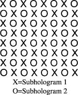
Figure 16.9. Interlacing scheme 2 with two subholograms.

In the IT method, once the entire hologram is divided into smaller subholograms, the first subhologram is designed to reconstruct the desired image f ðm; nÞ. The reconstructed image due to the first subhologram is h1ðm; nÞ. Because the subhologram cannot perfectly reconstruct the desired image, there is an error image e1ðm; nÞ defined as

In order to eliminate this error, the second subhologram is designed with e1ðm; nÞ=l1 as the desired image. Since the Fourier transform is a linear operation, the total reconstruction due to both subholograms is simply the sum of the two individual reconstructions. If the second subhologram was perfect and its scaling factor matched l1, the sum of the two reconstructed images would produce f ðm; nÞ. However, as with the first subhologram, there will be error. So, the third subhologram serves to reduce the left over error from the first two subholograms. Therefore, each subhologram is designed to reduce the error between the desired image and the sum of the reconstructed images of all the previous blocks. This procedure is repeated until each subhologram has been designed.

Each subhologram is generated suboptimally by the POCS algorithm (other methods can also be used). However, the total CGH may not yet reach the optimal result even after all the subholograms are utilized once. To overcome this problem, the method is generalized to the IIT.

The IIT is an iterative version of the IT method, which is designed to achieve the minimum MSE [Ersoy, Zhuang and Brede, 1992]. The reconstruction image of the ith subhologram at the jth iteration will be written as hjiðm; nÞ. After each subhologram has been designed using the IT method, the reconstruction due to the entire hologram hf ðm; nÞ has a final error ef ðm; nÞ. To apply the iterative interlacing technique, a new sweep through the subholograms is generated. In the new sweep,

Figure 16.11. The binary hologram generated with the IIT method for the cat brain image.

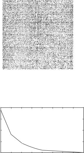
Figure 16.11 shows the binary hologram generated with the IIT method for the cat brain image. Figure 16.12 shows how the error is reduced as a function of the number of iterations. Figure 16.13 shows the corresponding He–Ne laser beam reconstruction.

Iteration number

Figure 16.12. Error reduction as a function of iteration number in IIT design.

Figure 16.15. Interlacing of subholograms in ODIFIIT with m ¼ n ¼ 2.

conjugate of the reconstructed image exists in the region Rþ due to the real-valued CGH transmittance. Since the binary CGH has cell magnitude equal to unity, it is important that the desired image is scaled so that its DFT is normalized to allow a direct comparison to the reconstructed image hðm; nÞ.

The total CGH is divided into m n subholograms, or blocks, where m ¼ M=A and n ¼ N=B: m and n are guaranteed to be integers if M, N, A, and B are all powers of two. Utilizing decimation-in-frequency [Brigham, 1974], the

Defining Hðk; lÞ as the sum of all the subholograms, the expression for the reconstructed image becomes

where 0 m < M, 0 n < N.

The reconstructed image in the region R is computed by replacing m and n by m þ M1 and n þ N1, respectively, and letting m and n span just the image

region:

hðm þ M1; n þ N1Þ

where 0 m A 1, 0 n B 1.

Let ha;bðm; nÞ be the size A B inverse discrete Fourier transform of the ða; bÞth subhologram:

ha;bðm; nÞ ¼ IDFTAB½Hðmk þ a; nl þ bÞ&m;n

where 0 a m 1, 0 b n 1, 0 m A 1, 0 n B 1.

Using the IDFT of size A B, the reconstructed image inside the region R becomes

the size A B IDFTs of all the subholograms. From this equation, it can be seen that the reconstructed image in the region R due to the ða; bÞth subhologram is given by

which is the IDFT of the ða; bÞth block times the appropriate phase factor, divided by mn.

An array, which will be useful later on, is defined as follows:

~ ð þ þ Þ ¼ ð þ þ Þ 0 ð þ þ Þ ð Þ ha;b m M1; n N1 h m M1; n N1 ha;b m M1; n N1 : 16:5-6

This is the reconstructed image in the region R due to all the subholograms except the ða; bÞth subhologram.

Conversely, given the desired image in the region R, the transmittance values can be obtained. From Eq. (16.5-2)

where 0 k A 1, 0 l B 1, 0 a m 1, 0 b n 1:

Therefore, the transmittance values of the subhologram ða; bÞ that create the image hðm þ M1; n þ N1Þ in the region R are given by

h i

Hðmk þ a; nl þ bÞ ¼ WA M1kWB N1lDFTAB hðm þ M1; n þ N1ÞWMðmþM1ÞaWN ðnþN1Þb

k;l

ð16:5-9Þ

where 0 k A 1, 0 l B 1:

Using Eqs. (16.5-5) and (16.5-9), we can compute the reconstructed image in the region R due to each individual subhologram, or, given a desired image in the region R, we can determine the transmittance values needed to reconstruct that desired image. Therefore, we can now utilize the IIT to design a CGH.

Letting f0ðm þ M1; n þ N1Þ, 0 m A 1, 0 n B 1, be the the desired image of size A B, the ODIFIIT algorithm can be summarized as follows:

1.Define the parameters M, N, A, B, M1, and N1, and determine m and n. Then, divide the total CGH into m n interlaced subholograms.

2.Create an initial M N hologram with random transmittance values of 0 and 1.

3.Compute the M N IDFT of the total hologram. The reconstructed image in

the region R is the points inside the region R, namely, hðm þ M1; n þ N1Þ, 0 m A 1, 0 n B 1.

4.The desired image f ðm þ M1; n þ N1Þ is obtained by applying the phase of each point hðm þ M1; n þ N1Þ to the amplitude f0ðm þ M1; n þ N1Þ as in the POCS method. So,

where fmþM1;nþN1 ¼ argfhðm þ M1;n þ N1Þg.

is the reconstructed image in the region R due to all the subholograms except the ða; bÞth subhologram.

7.Determine the error image that the ða; bÞth subhologram uses to reconstruct (i.e., the error image) as

which is equivalent to the error image in the IIT method.

8.Using Eq. (16.5-9), find the transmittance values Eðmk þ a; nl þ bÞ for the current block that reconstructs the error image.

9.Design the binary transmittance values of the current block as

10. Find the new reconstructed image h0a;bðm þ M1; n þ N1Þ in the region R due to the current block.

11. Determine the new total reconstructed image hðm þ M1; n þ N1Þ by adding

0 ð þ þ Þ ~ ð þ þ Þ the new ha;b m M1; n N1 to ha;b m M1; n N1 .

12. With the new hðm þ M1; n þ N1Þ, use Eq. (16.5-10) to update f ðm þ M1;

n þ N1Þ.

13.Repeat steps 7–12 until the transmittance value at each point in the current block converges.

14.Update the total hologram with the newly designed transmittance values.

15.Keeping l the same, repeat steps 3–14 (except step 5) for all the subholograms.

16.After all the blocks are designed, compute the MSE from Eq. (16.3-7).

17.Repeat steps 3–16 until the MSE converges. Convergence indicates that the optimal CGH has been designed for the current l.

16.5.1Experiments with ODIFIIT

The ODIFIIT method was used to design the DOEs of the same binary E and girl images that were used in testing Lohmann’s method. There two images are shown in Figure 15.3 and Figure 15.8, respectively. A higher resolution 256 256 grayscale image shown in Figure 16.16 was also used.

The computer reconstructions from the ODIFIIT holograms are shown in Figures 16.17–16.19.

All the holograms designed using the ODIFIIT used the interlacing pattern as shown in Figure 16.15. There are many different ways in which the subholograms