

Solid-Phase Synthesis and Combinatorial Technologies
.pdf5.4 LIBRARY DESIGN VIA COMPUTATIONAL TOOLS 183
DISTANCES |
4-points |
|
pharmacophore |
||
|
3-points pharmacophore
ANGLES
CIRCLES MAY BE positive or negative charges, hydrogen bond donors or acceptors, lipophilicity centres, and so on
DISTANCES are in Angstroem; increments of distances/pharmacophore distances define the bins to be filled
ANGLES are in degrees; increments of angles/pharmacophore angles define the bins to be filled (see example below)
angle: 90°
angle: 120°
Figure 5.13 Three-dimensional molecular descriptors: several examples.
overall evaluation of the molecules and would overestimate the contribution of this property to the determination of global diversity for a virtual library. All classes of descriptors have proven useful to select diverse sets of compounds when compared to random selections (29), but the use of flexible 3D descriptors/pharmacophores for huge virtual libraries is, as of today, prevented by the computational time and memory required.
Any type of selected descriptor will provide a more or less complex characterization of each virtual library component. The use of similarity indices offers a straightforward method to evaluate similarities between virtual compounds. These indices use a bit-string representation for any descriptor (distances, fingerprints, pharmacophores, and so on) and, by simply counting the presence or the absence of specific bins and comparing the bit strings of virtual compounds, provide a numerical similarity index. The formula for the commonly used Tanimoto similarity index (71, 43), which can readily be transformed into the complementary diversity index, is reported in Fig. 5.14

184 SYNTHETIC ORGANIC LIBRARIES: LIBRARY DESIGN AND PROPERTIES
MOLECULE A (STANDARD)
|
|
|
|
|
|
|
|
|
|
|
|
|
|
|
|
|
|
|
|
MOLECULE B |
||
|
|
|
|
|
|
|
|
|
|
|
|
|
|
|
|
|
|
|
|
|
|
|
|
|
|
C |
C |
|
|
|
|
|
C C |
|
|
|
|||||||||
Tanimoto similarity index: |
|
|
|
|
Ncommon |
|
|
4 |
||||||||||||||
|
|
|
|
|
|
|
|
|
= |
= 0.2 |
||||||||||||
|
|
|
|
|
|
|
|
|
|
|
|
Ncommon + Ndifferent |
|
|
20 |
|||||||
|
|
|
|
|
|
|
|
|
|
|
|
|
|
|
|
Ndifferent |
|
|
16 |
|||
Tanimoto dissimilarity index: |
|
|
|
|
|
|
|
|
|
|
= |
= 0.8 |
||||||||||
|
|
|
|
|
|
|
|
|
|
|
|
|
|
Ncommon + Ndifferent |
|
|
20 |
|||||
Figure 5.14 Similarity/dissimilarity comparison of two molecules: the Tanimoto index.
(molecules A and B are highly dissimilar in this hypothetical example). Such an index, even if questionable when applied to dissimilarity evaluations (54), allows fast comparisons between structures or subsets of molecules.
Compound selection is a core process of library design, and three main methods can be mentioned. Dissimilarity-based methods select compounds in terms of similarity/distance between individuals in chemical space. Clustering methods first group compounds into clusters based on similarity/distance and then choose representative compounds from different clusters. Partitioning methods first create a uniform cell space that subdivides the “chemical space,” then assign all virtual compounds to the relative cells according to their properties, and finally choose representative compounds from different cells.
Dissimilarity-based methods are the fastest selection techniques, as can be easily seen from the hypothetical example reported in Fig. 5.15. This method, based on the maximum dissimilarity approach (72–74), must first define a minimum acceptable dissimilarity threshold R and a maximum subset M of compounds to be selected. The paradigm starts randomly from any virtual component (A, Fig. 5.15) and then searches for the most dissimilar individual in the virtual population (B, Fig. 5.15). The following selection rounds choose the individual most dissimilar from all those already selected, and this process is repeated (A–E, Fig. 5.15) until either the last selection produces a candidate whose dissimilarity to the other selected components is less than R or until M number of virtual components (five in the example) have been selected. Such a method is easy and fast, does not require significant computing time, and, while intrinsically biased toward picking extreme compounds from a virtual library (73), allows reasonably diverse selections even in very large virtual libraries. Other dissimilarity-based selection methods, which can complement nicely the maximum dissimilarity approach, have been reported in the past few years (75–77); their performance in

|
5.4 |
LIBRARY DESIGN VIA COMPUTATIONAL TOOLS 185 |
|||
x |
|
x |
|
x |
x |
|
|
B |
|||
|
D |
|
|
|
|
|
|
|
|
x |
|
|
x |
x |
|
|
x |
|
|
|
|
||
x |
x |
|
|
x |
|
|
|
|
x |
||
|
|
|
|
|
|
x |
|
x |
|
|
|
|
|
|
x |
E |
|
x |
|
|
|
x |
|
x |
|
|
|
||
|
x |
|
x |
x |
|
|
|
|
|||
|
|
|
|
|
|
|
|
x |
x |
|
x |
x |
A |
|
|
x |
|
|
|
|
|
C |
|
CHEMICAL SPACE: maximum dissimilarity method
Figure 5.15 Dissimilarity-based selection methods: maximum dissimilarity approach.
selecting active compounds has been recently compared using available databases of drug molecules (78).
The clustering method (79–81) first groups the virtual library components in clusters, such that all the individuals belonging to the same cluster have a high similarity and the individuals in different clusters have a high degree of dissimilarity. Each cluster may contain many compounds or even just one compound, called a singleton. The purpose of clustering is to select the most representative set of diverse compounds, composed of a relatively small number of individuals: A method that reduces the number of singleton clusters is highly recommended. One class of clustering methods is called nonhierarchical, an example of which is depicted in Fig. 5.16. To begin with, a search of the nearest neighbors (the most similar compounds to the selected structure in the virtual set) is performed for two compounds (A and B, Fig. 5.16) and a previously defined number X of nearest neighbors (8, included in circles, for A and B). Both compounds must be in each others nearest-neighbor sets (B in A’s neighbors and A in B’s neighbors), and a predefined minimum number of virtual compounds must be present in both neighbors sets (5 out of 8, including A and B, in Fig. 5.16: compounds in bold characters). If these conditions are satisfied, as for A and B in the example, the two compounds are clustered together. If a compound is not among the nearest-neighbor set of another (as C for B, Fig. 5.16), or if the minimum number of shared nearest neighbors is not satisfied (as C for A, being only 4 out of 8 in common), the compounds are considered members of two different clusters. This strategy does not take into account the relationship between different clusters, limiting its usefulness, and usually gives high numbers of singletons, which makes the selection of small sets more complex, but it is fast and useful for very large sets of virtual libraries. The so-called Jarvis–Patrick (82, 83) clustering technique is the most commonly used and has been applied to several compound selections (84, 40). Another
186 SYNTHETIC ORGANIC LIBRARIES: LIBRARY DESIGN AND PROPERTIES
x |
x x |
x |
x x |
|
|
||
x |
x |
x |
x |
x |
|
x x |
|
x |
|
|
x |
x |
|
|
|
x x x |
x |
x |
|
C |
x |
||
x |
x |
x x |
x |
x |
|
||
x x |
x |
x |
x |
x x A |
|
||
x |
x |
x |
x |
|
B x |
||
x |
x |
x x |
x x |
x |
|
||
CHEMICAL SPACE: non-hierarchical clustering
Figure 5.16 Clustering selection methods: nonhierarchical approaches.
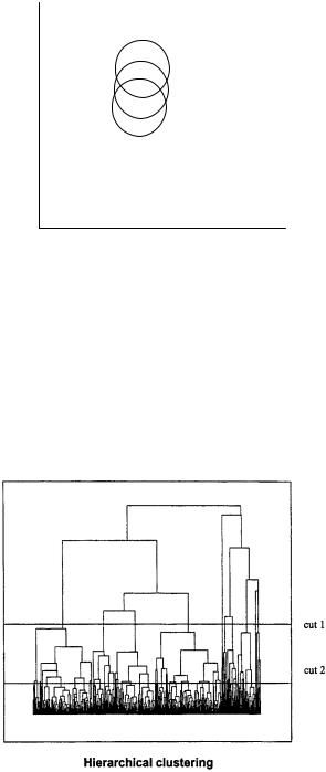
class of clustering methods, called hierarchical methods, provides parent–daughter relationships between clusters and allows clustering according to the selection needs; an example of these methods is shown in Fig. 5.17. The treelike dendrogram can be cut at any level to give clusters of different number and size as necessary (cut 1, 10 clusters; cut 2, 32 clusters; Fig. 5.17). The dendrograms can be generated from the first huge cluster either by going to the highest fragmentation (hierarchical) or by working
Figure 5.17 Clustering selection methods: hierarchical approaches.
5.4 LIBRARY DESIGN VIA COMPUTATIONAL TOOLS 187
from the bottom up (agglomerative). These methods are more information rich than the nonhierarchical techniques but are also significantly more computationally time consuming. A popular hierarchical technique, the Ward method (85), has been used frequently for compound selections (84, 86, 87). Clustering methods, while outperforming dissimilarity-based methods, are generally computationally time consuming and arbitrary, measuring diversity among a given virtual set without framing it in the chemical space generated by the selection descriptors; nevertheless successful applications of clustering protocols to medium–large databases are made by known druglike compounds and library individuals (88). It is difficult to add new virtual compounds designed to increase the set diversity using clustering because a total reclustering process should be performed after each compound addition.
Partitioning methods (89–91) first subdivide chemical space into predefined bins (Fig. 5.18) by simply defining incremental values of the descriptors used and then assign each virtual library component to its proper bin. The schematic examples in Fig. 5.18 consider two properties/descriptors Y (8 increments, A–H) and X (12 different increments, 1–12) that generate 96 different bins, or cells. The library partitioned in Fig. 5.18, top, is clearly diverse, spanning the large majority of the bins, while underneath we have a library containing a large number of compounds in a small area of chemical space producing a nondiverse library. These methods, compared to clustering, are less computationally demanding and allow a better evaluation of a library in terms of diversity. In fact, the voids in the space are evident (see Fig. 5.18), and additional virtual compounds can be designed to fit into the desired bin. As a drawback, very similar compounds can sometimes fall into two different cells: for example, if the molecular weight is one of the considered properties and two increments are 200 < MW < 300 and 300 < MW < 400, two compounds weighing respectively 299 and 301 daltons would occupy two different bins. Recent examples of large library diversity analysis by partitioning techniques have been reported (92, 93).
In general, dissimilarity-based selections are less time and computationally consuming but are also less accurate in predicting and/or selecting diverse sets; clustering methods are good when large agglomerations of similar compounds are present in the virtual set, as they discriminate well among them; partitioning methods are reasonably fast and effectively represent large varied sets of virtual candidates. It is very difficult to give absolute rules regarding the best choice in terms of descriptors, indices, and selection methods to select the most diverse libraries: This process is highly project specific, and the best solution readily changes from case to case. However, as mentioned earlier, it has been thoroughly proven that a selection using computational diversity/similarity analysis (see also the next Section) is more successful than a random selection in producing a more meaningful library.
5.4.2 Focused Libraries
We could say that it is enough to substitute the concept of dissimilarity with that of similarity in the previous section to determine the application of computational library design to focused libraries. In fact, the tools used to describe and to select among virtual

188 SYNTHETIC ORGANIC LIBRARIES: LIBRARY DESIGN AND PROPERTIES
|
|
|
|
|
|
|
CHEMICAL SPACE |
|
|
|
|
|
|
|
|
|||||||
|
|
|
|
|
|
|
|
|
|
|
|
|
|
|
|
|
|
|
|
|
|
|
H |
|
|
x |
|
|
|
|
x |
|
|
|
|
x |
|
|
|
|
x |
|
x |
|
|
|
|
|
|
|
|
|
|
|
|
|
|
|
|
|
|
|
|
|
|
|
x |
|
|
|
|
|
|
|
x |
|
|
|
x |
|
|
|
|
x |
|
|
|
|
|
|
|
|
|
|
|
|
|
|
|
|
|
|
|
|
|
|
|
x |
|
|
|
|
||
|
|
|
|
|
|
|
|
|
|
|
|
|
|
|
|
|
|
|
|
|
||
|
|
|
|
|
|
|
|
|
|
|
|
|
|
|
|
|
|
|
|
|
|
|
|
|
|
x |
|
|
x |
|
|
|
|
|
|
x |
|
|
|
|
|
x |
|
|
|
|
|
|
|
|
|
|
|
|
|
|
|
|
|
|
x |
|
x |
|
||||
|
|
|
|
|
|
|
|
|
|
|
|
|
|
|
|
|
|
|
||||
|
|
|
|
|
|
|
|
|
|
|
|
|
|
|
|
|
|
|
|
|
||
|
|
|
x |
|
|
|
|
x |
|
|
|
|
|
|
|
|
|
|
|
|
|
|
|
|
|
|
|
|
|
|
|
|
|
|
x |
|
|
|
x |
|
|
x |
|
|
|
|
|
|
x |
|
x |
|
|
|
x |
|
|
x |
|
|
x |
|
x |
|
|
|
|
|
|
|
|
|
|
|
|
|
|
|
|
|
|
|
|
|
|
|
|||||
|
|
|
|
|
|
|
|
|
|
|
|
|
|
|
|
x |
|
|
|
|||
|
|
x |
|
|
|
|
|
|
|
|
|
|
|
|
|
|
|
|
|
|
||
|
|
|
|
|
|
|
|
|
|
|
|
|
|
|
|
|
|
|
|
|||
|
|
|
|
|
|
|
|
|
|
|
|
|
|
|
x |
|
|
|
|
|
|
|
A |
|
|
x |
|
x |
|
|
|
|
|
x |
|
|
|
|
x |
|
|
|
|
||
|
|
|
|
|
|
|
|
|
|
|
|
|
|
|
|
|
|
|||||
|
|
|
|
|
|
|
|
|
|
|
|
|
|
|
|
|
|
|||||
|
|
|
|
|
|
|
|
|
|
|
|
|
|
|
|
|
|
|
|
|
|
|
|
1 |
|
|
|
|
|
|
|
|
|
|
|
|
|
|
|
|
12 |
|
|
||
|
|
|
|
|
PARTITIONING PROTOCOLS: |
|
|
|
|
|
|
|||||||||||
|
|
|
|
a diverse set (top) and a similar set (bottom |
|
|
|
|
||||||||||||||
|
|
|
|
|
|
CHEMICAL SPACE |
|
|
|
|
|
|
|
|
||||||||
H |
|
|
|
|
|
|
|
|
|
|
|
|
|
|
|
|
|
|
|
|
|
|
|
|
|
|
|
|
|
|
|
|
|
|
|
|
|
|
|
|
|
|
|
|
|
|
|
|
|
|
|
|
|
|
|
|
|
|
|
|
|
|
|
|
|
|
|
|
|
|
|
|
|
|
|
|
x |
x x |
x |
x |
x |
x |
|
|
|
|
|
|
|||
|
|
|
|
|
|
|
x |
x |
x |
x |
x |
|
|
|
|
|
|
|||||
|
|
|
|
|
|
x |
x |
x |
x |
x |
x |
|
|
|
|
|
|
|||||
|
|
|
|
|
|
x x |
|
|
|
|
|
|
||||||||||
|
|
|
|
|
|
|
|
|
x |
|
x |
x x |
|
|
|
|
|
|
||||
|
|
|
|
|
|
|
|
x |
x |
x |
x |
|
|
|
|
|
|
|
|
|||
|
|
|
|
|
|
|
|
x |
|
|
|
|
|
|
|
|
|
|
|
|
|
|
|
|
|
|
|
|
|
x x |
x |
x |
x |
x x x |
|
|
|
|
|
|
|||||
|
|
|
|
|
|
|
x |
x |
x |
x |
x x |
|
|
|
|
|
|
|||||
|
|
|
|
|
|
|
|
x |
|
x |
|
x |
x x |
x |
|
|
|
|
|
|
||
|
|
|
|
|
|
|
|
|
|
|
x |
|
|
|
|
|
|
|
|
|
|
|
A
1 |
12 |
Figure 5.18 Partitioning selection methods: diverse (top) and similar (bottom) sets of compounds.
molecules may be the same as seen previously, while the goal is now to find the most similar sets of reagents/products to produce a library similar in respect to a known structure (compound A, Fig. 5.19), or to a structural hypothesis (e.g., fit into a pharmacophore). We should always remember, though, that chemical and biological diversity, or similarity, are not the same thing. Very similar structures may have a

|
|
|
|
5.4 |
LIBRARY DESIGN VIA COMPUTATIONAL TOOLS 189 |
|||||||
x |
|
x |
|
x |
|
x |
|
x |
x |
|
|
|
|
|
|
x |
x |
x |
x |
|
|||||
|
|
|
|
x |
|
x |
||||||
|
x |
|
x |
x |
x |
x |
x |
x |
x |
|||
|
|
|
|
|||||||||
|
|
|
|
|
x |
x x |
x |
x |
x x |
|||
x |
|
|
|
|
|
x |
x |
|
|
x x |
||
x |
|
|
x |
|
x |
x A x x |
|
|||||
|
|
|
x |
x |
|
|||||||
|
|
|
|
|
|
x |
x |
x |
x x x |
|||
x |
|
x |
|
|
|
x x x |
x |
x |
x |
|
x x |
|
|
|
|
|
x |
|
x |
x |
|
x |
x x |
x |
|
x |
|
|
|
|
x |
|
|
x |
|
|
|
|
x |
|
|
|
x |
|
|
|
|
|
|
||
|
|
x |
x |
|
|
|
|
|
|
|
||
|
|
|
|
|
|
|
|
|
|
|||
|
|
|
|
|
|
|
|
|
|
|
|
|
|
|
x |
|
x |
x |
|
|
|
|
|
|
|
x |
|
|
|
|
|
|
|
|
|
|
|
|
|
CHEMICAL SPACE: |
|
|
|
|
CHEMICAL SPACE: |
||||||
|
|
diverse library |
|
|
|
|
|
focused library |
||||
Figure 5.19 Chemical similarity in the chemical space.
Tanimoto index > 0.9 but may be very different in terms of activity (chemically similar, biologically diverse), while completely different structures are known to have the same biological activity (chemically diverse, biologically similar). This intrinsic drawback to the computational screening of virtual libraries should always be considered when interpreting screening results of a computationally designed library, and real data should be used to refine any virtual SAR information based on chemical similarity or dissimilarity.
The number of individuals in a focused library is usually small so that it is easy to rapidly design a small set, then prepare and test it. Once this preliminary quantitative structure activity relationship (QSAR) is known, the available information can be used to produce a more significant second focused library, and the iterative cycle can continue until an active product with the desired potency is obtained. A few other points are worth mentioning. The significantly smaller set of virtual library components usually allows the use of 3D descriptors, especially as threeor four-point pharmacophores. Rather than using similarity/dissimilarity indices, such as Tanimoto’s, the comparison of fingerprints/pharmacophores can be carried out and even stored in most cases. The virtual focused library will contain mostly clusters of very similar individuals, and clustering becomes the selection method of choice where the similarity parameters can be tailored so as to obtain highly diversified subsets.
Four recent examples of computational selection of the most similar compounds in a virtual library set will be now reviewed. Either a few different lead structures were available as starting points for the selection or a detailed knowledge of the target allowed to design and select a medium/small focused library.
The first two examples, which imply that similarity between compounds is related to similar activity profiles, use two popular selection methods: genetic algorithms (GA; 96–100) and simulated annealing (SA; 101, 102).
Pentapeptides were used (94) as a training set for the design of bradykinin-poten- tiating peptides. The two known active sequences 5.1 and 5.2 (103, 104) were used to


|
|
|
|
|
|
5.4 LIBRARY DESIGN VIA COMPUTATIONAL TOOLS |
191 |
|||||||||||||
|
|
|
|
|
|
|
|
AA2 |
AA4 |
|
|
|
|
AA |
2 |
|
AA |
|
||
|
AAx |
AAx |
|
|
|
AA1 |
AA3 |
AA5 |
|
AA |
|
|
|
|
9 |
|
||||
|
|
|
|
|
1 |
|
|
AA |
AA |
|
||||||||||
AAx |
AAx |
AAx |
|
|
|
|
|
|
|
|
|
|
|
3 |
10 |
|
||||
a |
|
27 |
|
|
b |
|
|
|
|
101 |
|
|
||||||||
|
|
|
|
|
|
|
|
|
|
|
|
|
|
|
||||||
1-100 |
|
|
|
|
|
|
|
|
|
|
|
|
|
|
|
|
|
|||
|
|
|
|
|
|
|
|
|
|
|
|
|
|
|
|
|
||||
|
|
|
|
|
|
|
|
|
|
|
|
|
|
|
|
|
||||
|
randomly |
|
|
|
|
AA7 |
AA9 |
|
|
|
|
AA |
7 |
|
AA |
|
||||
selected pentapeptides |
|
AA6 |
AA8 |
AA10 |
AA |
|
|
|
|
4 |
|
|||||||||
|
6 |
|
|
AA |
8 |
AA |
|
|||||||||||||
|
|
|
|
|
|
|
|
74 |
|
|
|
|
|
|
|
5 |
|
|||
|
|
|
|
|
|
|
|
|
|
|
|
|
|
|
|
102 |
|
|
||
|
|
|
|
|
|
|
|
|
|
|
|
|
|
|
|
|
|
|
||
|
|
|
|
|
|
|
|
|
|
|
AAx |
|
|
AAx |
|
|
|
|
|
|
|
|
|
|
|
|
|
|
|
AAx |
|
AAx |
|
AAx |
|
|
|
||||
|
|
|
|
AA2 |
|
AA9 |
d |
|
|
1-100 |
|
|
|
|
|
|
||||
|
|
|
|
|
negative evolution |
|
|
|
||||||||||||
|
c |
AA1 |
|
|
AA3 |
AA10 |
|
|
|
|
|
|
|
|
|
|
|
|
||
|
|
|
|
101 |
|
|
|
|
|
|
|
|
|
|
|
|
|
|
||
|
|
|
|
AAx |
|
AA4 |
e |
|
|
AAx |
|
|
AAx |
|
|
|
|
|
||
|
|
|
|
|
|
|
|
|
|
|
|
|
|
|||||||
|
|
|
AA6 |
|
|
AA8 |
AA5 |
|
|
|
|
|
|
|
|
|
||||
|
|
|
|
|
AAx |
|
AAx |
AAx |
|
|
|
|||||||||
|
|
|
|
103-121 |
|
|
|
|
|
|||||||||||
|
|
|
|
|
1-26, 28-73, 75-100, 102, 114 |
|
|
|||||||||||||
|
|
|
|
|
|
|
|
|
|
|
||||||||||
|
|
|
|
|
|
|
|
|
positive evolution |
|
|
|
|
|||||||
f
AAx AAx
AAx |
AAx |
AAx |
genetically selected, most similar pentapeptides
a: random selection; b: crossover; c: single point mutation; d,e: selection of the two best scoring sequences among 27, 74 and 101-121; f: repeat a-e (2000 times).
Figure 5.21 GA-based selection: a detailed protocol for a 3,200,000-membered pentapeptide virtual library.
100-membered population of similarity-based pentapeptides. In the reported example, the 100 most similar pentapeptides generated after 2000 iterations bore a striking resemblance to the 100-membered set generated after exhaustive comparison of all the 3,200,000 virtual pentapeptides. The amino acid composition for each position was almost identical for the final GA iteration and for the exhaustive search of the virtual set. This impressive result, which derived from the use of topological descriptors related to the properties of the whole pentapeptides for similarity comparisons (the reagent-based descriptors performance was significantly worse), was possible because only several thousands of structures were considered and evaluated during the 2000
