The Elisa guidebook

Page 313

distribution statistic in both types of population and that a representative sampling procedure for the whole population is being measured. The rationale here is that approx 95% of normally distributed observations are expected to fall within a range of mean 2 ¡Á SD, and would test negative. However, as already indicated, the normal distribution is not always realized, and the distribution of positives (particularly) is neglected. This may be, and often is, biased. The major flaw in this method is that it deals with the specificity of the assay results but not the sensitivity. The value can be regarded as a good reference value. The continuous validation of assays, with reference to evaluating a wider number of epidemiological niches using the same reagents, often modifies the cutoff value using this criterion. The relationship between sensitivity and specificity cannot be forgotten in any consideration. Raising the cutoff value increases specificity, and reducing it increases diagnostic sensitivity (reduces specificity). Whether this matters depends on the problem being tackled, and what types of results can be accepted. For example, false positive results may be unacceptable. This is true in, say, in the diagnosis of AIDS. However, it is important that someone not be missed either. False negative results may be acceptable in cases in which another test can be used in parallel. The first screening of samples could be with an ELISA set to have low sensitivity, but would be specific and reduce the number of clear positives, to relieve the burden on another more sensitive assay (e.g., polymerase chain reaction [PCR]).

Borderline or intermediate results require cautious in interpretation. Statistically this gray zone defines a range of cutoff values that would result in a sensitivity or specificity less than a predefined level. Although there are techniques to attempt to compensate for unknown factors, the best approach is to assimilate as much data from all sources. This allows explanation and then manipulation (selection) of data to help eliminate bias. The flexibility in altering the cutoff value is data dependent and a continuous process in test validation.

1.8¡ª

Calculation of D-SN and D-SP: Predictive Value of Diagnostic Tests

The inferences from test results rather than observed test values are of interest to the diagnostician. Thus, the use of the assay rather than the technology itself is key. Measurement of disease state, level of protective antibody, and transition of disease status are all objectives. Rarely is there a perfect correlation between disease status and any test result. Thus, there is always some degree of false positivity or negativity. The establishment of the correlation is regarded as diagnostic evaluation. The standard for presenting such results is in Table 1, which relates true positive (TP), true negative (TN), false positive (FP), and false negative (FN) results represented as frequencies of the four possible decisions. These can be shown in a 2 ¡Á 2 (see Table 1).

Page 314

Table 1

Relationships of Disease

Status and Test Resultsa

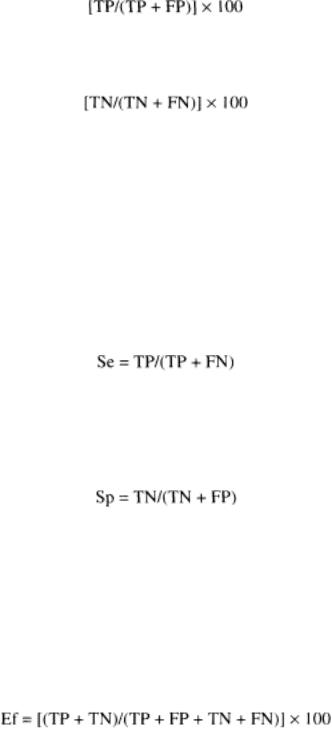
aDiagnostic (clinical) sensitivity = [TP/(TP + FN)] ¡Á 100. Diagnostic (clinical) specificity is [TN/ (TN + FP)] ¡Á 100.

D-SN and D-SP can be estimated from test results on a panel of reference sera chosen early in the validation process. Calculations of D-SN and D-SP, therefore, only apply to the reference sera and can be extrapolated to the general population of animals only insofar as the reference sera fully represent all variables in that targeted population. The paramount importance of the proper selection of reference sera is thus self-evident.

Other terms based on these values can be defined as follows.

1.8.1¡ª

Prevalence of Disease (P)

Prevalence of disease denotes the probability of a subject as having a disease:

P is an unbiased estimator of the prevalence in a target population if animals can be randomly selected and subjected to both the reference test (to establish D) and the new test (T).

1.8.2¡ª

Apparent Prevalence

Apparent prevalence (AP) denotes the probability of a subject to have a positive test result:

1.8.3¡ª Predictive Value

The predictive value of a positive test gives the percentage of subjects suffering from disease correctly classified as positive by the test, and defined as follows:

Page 315

The predictive value of a negative test gives the percentage of healthy subjects correctly classified as negative by the test, and defined as follows:

1.8.4¡ª

Components of Diagnostic Accuracy

Accuracy is the ability of a test to give correct results (diagnostic sensitivity). As already indicated, this can be estimated by the observed agreement of the new and reference test. There are two components.

1.8.4.1¡ª Sensitivity

Sensitivity (Se) is the probability of a positive result (T+) given that the disease is present (D+):

1.8.4.2¡ª Specificity

Specificity (Sp) is the probability of a negative results (T¨C) given that the disease is not present (D¨C):

1.9¡ª

Combined Measures of Diagnostic Accuracy

1.9.1¡ª Efficiency

The overall efficiency (Ef) of a diagnostic test, defined as the percentage of subjects correctly classified as diseased or healthy, with a given prevalence of P, is estimated using the following relationship:

1.9.2¡ª Youden's Index

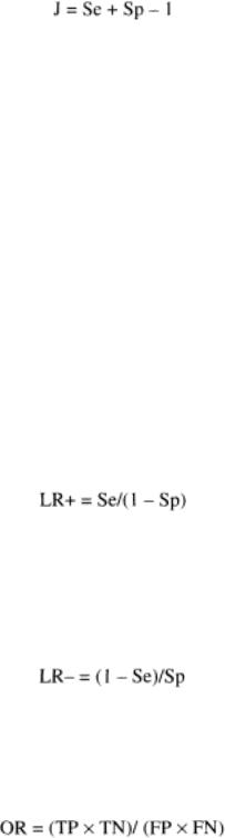
Youden's Index (J) is the measure of the probability of correct classifications that is invariant to prevalence. In terms of Se and Sp we have:

1.9.3¡ª Likelihood Ratios

Likelihood ratios (LRs) are important measures of accuracy that link estimations of preand posttest accuracy. They express the change in likelihood of disease based on information gathered before and after making tests. The degree of change given a positive result (LR+) and given a negative result (LR¨C) depends on the SDe and Sp of the test.

Page 316

1.9.3.1¡ª

Likelihood Ratio of a Positive Test Result

The likelihood ratio (LR) of a positive test result is the ratio of the probability of disease to the probability of nondisease given a positive test result, divided by the odds of the underlying prevalence [odds (P) = (P/1 ¨C P)]:

1.9.3.2¡ª

Likelihood Ratio of a Negative Test Result

The likelihood ratio of a negative test result is the ratio of the probability of disease to the probability of nondisease given a negative test result, divided by the odds of the underlying prevalence:

1.9.3.3¡ª Odds Ratios

Odds ratios (ORs) combine results from studies:

1.10¡ª

Examples Relating Analytical and Diagnostic Evaluation

In a new ELISA, 250 sera have been examined from nonexposed animals and 92 infected animals. Table 2 presents the results.

The following data reflect some of the features already discussed:

ROC analysis was developed in the early 1950s and extended into medical sciences in the 1960s. It is now a standard tool for the evaluation of clinical tests. The underlying assumption in ROC analysis is that the diagnostic variable is to be used as the discriminator of two defined groups of responses (e.g., test values from diseased/nondiseased animals, or infected/noninfected animals). ROC analysis assesses the performance of the system in terms of Se and 1 ¨C Sp for each observed value of the discriminator variable assumed as a decision threshold, e.g., cutoff value to differentiate between two groups of responses. For ELISA, which produces continuous results, the cutoff value can be shifted over a range of observed values, and Se and 1 ¨C Sp are established for each of these. Setting this as k pairs, the resulting k pairs ([1 ¨C Sp] Se) are displayed as an ROC plot. The connection of the points leads to a trace that originates in the upper right corner and ends in the left lower corner of the unit square. The plot characterizes the given test by the trace in the unit square, irrespective of the original unit and range of the measurement. Therefore, ROC plots can be used to compare all tests, even when the tests have quite different cutoff values and units of measurement. ROC plots for diagnostic assays with perfect discrimination between negative and positive reference samples pass through coordinates (0; 1), which is equivalent to Se = Sp = 100%. Thus, the area under such ROC plots would be 1. 0, and the study of the area under the curve (AUC), which evaluates the probabilities of (1 ¨C Sp) and Se, is the most important statistical feature of such curves.

1.11.1¡ª

Area under the ROC Curve

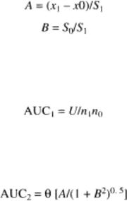
The theoretical exponential function underlying the ROC plot is estimated on the assumption that data from two groups are distributed normally (bimodally). The ROC function is then characterized by parameter A (standardized mean difference of the responses of two groups) and the parameter B (ratio of SDs). Thus, for a set of data for a positive and negative reference group with means of x0 and x1, in which x0 < x1 and the SDs are s0 and s1, respectively,

Page 318

The AUC can be estimated making assumptions about the distribution of test results. Therefore, a nonparametric test is based on the fact that the AUC is related to the test statistic U of the MannWhitney rank sum test:

With U = n1n0 + n0 (n0 + 1) / 2 ¨C R, R = rank sum of squares.

A parametric approach can be taken. Here,

Here we can see that for AUC = 0.5, then A = 0. Equal values for negative and positive reference populations indicate a noninformative diagnostic test. Theoretically, AUC < 0.5 if A is negative. In practice, such situations are not encountered, or the decision rule is converted to obtain positive values for A.

The bimodal distribution may not be justified for a given set of data, and other methods have been developed based on maximum likelihood estimates of the ROC function and the AUC.

1.11.2¡ª

Optimization of Cutoff Value Using ROC Curves

The optimal pair for sensitivity and specificity is the point with the greatest distance in a Northwest direction, from the diagonal line Se = (1 ¨C Sp) (see Figs. 2 and 3).

1.11.3¡ª

Example of ROC Analysis

The principle of ROC analysis is to generate plots using a spreadsheet (e.g., EXCEL) in which:

1.A grid of possible cutoff values is generated.

2.For each cutoff value, the resulting sensitivity (Se) and 1 ¨C Sp are calculated.

3.The values of Se are plotted against 1 ¨C Sp for all grid points.

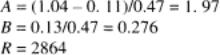
Many statistical packages can be used to construct ROC plots and shareware is available in the public domain. In this example (taken from ref. 1), the AUC is estimated for an ELISA for T3 using a test reference (T1), given the mean values of 1.04 and 0.11; the SDs 0.47 and 0.13; and the sample sizes 25 (positive subpopulation) and 75 (negative subpopulation). The rank sum and the U statistic are as follows:

Page 319

Fig. 2.

ROC plot for T3 data (T1 assumed as reference test, n = 100). Area under plot = 0.993; standard error (SE) = 0.012; 95% confidence interval

(CI) = 0.950¨C0.998.

We have stressed that an assay is valid only if the results of selected sera from reference animals represent the entire targeted population. Because of the extraordinary set of variables that may affect the performance of an assay, it is highly desirable to expand the bank of gold standard reference sera whenever possible. This follows the principle that variability is reduced with increasing sample size; therefore, increases in the size of the reference serum pool should lead to better estimates of D-SN and D-SP for the population targeted by the assay. Furthermore, when the assay is to be transferred to a completely differ-

Page 321

ent geographic region (e.g., from the Northern to Southern Hemisphere), it is essential to revalidate the assay by subjecting it to populations of animals that reside under local conditions. This is the only way to ensure that the assay is valid for that situation.

1.14¡ª

Assay Validation and Interpretation of Test Results

It is wrong to assume that a test result from a validated assay correctly classifies animals as infected or uninfected based solely on the assay's D-SN and D-SP. The calculations of D-SN and D-SP are based on testing the panel of reference sera and are calculated at one point in time. This is unlike the ability of a positive or negative test result to predict the infection status of an animal because this is a function of the prevalence of infection in the population being tested. Prevalence of disease in the target population, coupled with the previously calculated estimates of D-SN and D-SP, is used to calculate the predictive values of positive and negative test results.

For instance, assume a prevalence of disease in the population targeted by the assay of only 1 infected animal per 1000 animals, and a false positive rate of the test of 1 per 100 animals (99% D-SP). Of 1000 tests run on that population, 10 will be false positive and only 1 will be true positive. Therefore, when the prevalence of disease is this low, positive test results will be an accurate predictor of the infection status of the animal in only about 9% of the cases. Thus, if assay validation is concerned with accuracy in test results and their inferences, then proper interpretation of test results is an integral part of providing valid test results. It is beyond the scope of this chapter to discuss the many ramifications of proper interpretation of test results generated by a validated assay.

1.15¡ª

Validation of Assays Other Than ELISA

Although the example we have used was an indirect ELISA test, the same principles apply in the validation of any other types of diagnostic assay. Feasibility studies, assay performance characteristics, the size and composition of the animal populations that provide reference sera, and the continuing assessment and updating of the performance characteristics of the validated assay are all essential if the assay is to be considered thoroughly and continuously validated.