

The Elisa guidebook
.pdfFig. 2.
Plate layout for rinderpest competition ELISA. Controls are C++ (strong antibody positive); C+ (weaker antibody positive); Cm (mAb control, no sample); and C¨C
(conjugate control, no sample or mAb).
(nonprocessed) OD values, for each plate, are plotted for the Cm controls only on DDD charts and SDC charts. The PI% values are monitored for all controls on DDD and SDC charts. In terms of practical use of charts, a few rules can be given. These encourage the best use of the charts to allow easy monitoring and transparency of results to permit identification of problems on a continuous basis.
2.1¡ª
General Recommendations for Charting Methods
1.Charts should be displayed openly (on walls) and copies also kept on file.
2.A specific individual should be appointed to oversee the charts. This individual should ensure that all people performing the assays fill in the tables and chart the results. This individual should ensure that only relevant data are added to the charts, for example, plates used for developmental work or research should not be included, only those involved in running a routine assay.
3.The results on the charts should be discussed regularly with all involved in laboratory testing, and any trends identified and appropriate action taken.
2.2¡ª
Initial Examination of Kits
A great deal of care has been taken to ensure that the reagents and materials will work in laboratories worldwide with different local conditions, and that
Page 351
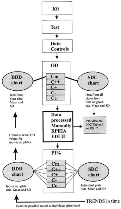
Fig. 3.
Scheme for plotting data on charts.
the kit will travel without deterioration of performance. On receipt of a kit, there are two initial questions: (1) How do we know that the kit reagents are

Page 352
Fig. 4.
Tables of Cm controls as OD values for DDD and SDC analysis.
Page 353

Fig. 5.
Table for data from Cm, C++, C+, C¨C, and Cc controls as PI%.
Page 354

Fig. 6.
Illustration of use of IQC Table 1 for obtaining DDD and SDC data.
Page 355

Fig. 7.
Illustration of use of IQC Table 2 for processing data.
Page 356
working as expected? and, (2) How can we ensure that the kit keeps on working, i.e., the established diagnostic criteria are maintained?
The first task then is to run an assay with the kit using available control reagents and to examine the results in the context of parameters given in the manual. This tells us whether the kit is performing as expected.
2.3¡ª
Running the Assay for the First Time
The following controls have been examined in the test. Test operators should familiarize themselves with the controls and their purpose. This information should be contained in the manual accompanying the kit.
Controls on ELISA plates are as follows:
1.Cm, mAb control.
2.C++, strong positive control.
3.C+, moderate positive control.

4.C¨C, negative serum control.
5.Cc, conjugate control (no serum/no monoclonal). Note the following conditions of the test:
1.The results expected (and the limits allowed) have been worked out by the suppliers of the kits.
2.These controls have been assessed many times and the results examined statistically.
3.The results using the control reagents have fixed limits.
4.If the results obtained are the same or within allowable limits, then your test is good.
5.If the results are outside the limits, then something is wrong.
2.4¡ª
Data Processing Fundamentals
Let us deal with the fundamentals of what the data processing does. Initial checks should determine that the controls have been placed in particular positions on the plate as shown in Fig. 2. A typical set of OD data for the controls is shown in Table 1. The data is processed to calculate PI% values and are shown in Table 2. The processing can be by hand (calculator) or through the use of dedicated software (as in the case of rinderpest ELISA). The formula for calculating the PI% value is as follows:
2.4.1¡ª
Calculation of Mean and Standard Deviation
The mean for each control sample is obtained by adding up all the individual values and dividing by the number of values used (the number of values is usually ascribed the letter n). The sign for the average (mean) is  . Thus, for the previously cited example, the mean OD for the Cm is 0.455 + 0.612 + 0.533 + 0.655 = 2.255 ¡Â 4 = 0.564.
Page 357
Table 1
Data for Control Sera on
One Plate
Control Data(OD)
Cc 0.010(0.009)
C++ 0.077(0.063)
C++ 0.072(0.071)
C+ 0.278(0.296)
C+ 0.313(0.280)
Cm 0.685(0.673)
Cm 0.636(0.641)
C¨C 0.668(0.667)

Table 2
Control Samples Data After Processing
|
OD1 |
OD2 |
OD3 |
OD4 |
PI%1 |
PI%2 |
PI%3 |
PI%4> |
C++ |
0.077 |
0.063 |
0.072 |
0.071 |
88 |
90 |
89 |
89 |
C+ |
0.278 |
0.296 |
0.313 |
0.280 |
58 |
55 |
52 |
57 |
C¨C |
0.668 |
0.667 |
¡ª |
¡ª |
¨C2 |
¨C2 |
¡ª |
¡ª |
Cc |
0.011 |
0.09 |
¡ª |
¡ª |
98 |
99 |
¡ª |
¡ª |
Cm |
0.685 |
0.673 |
0.636 |
0.641 |
¨C4 |
-2 |
¨C9 |
¨C8 |
The standard deviation (SD) in mathematical terms is the positive square root of the variance of the data. The variance is measured by subtracting the mean of the test wells data ( 1,
1,  2,
2,  3, and so on) from the overall mean value (X) and squaring that value. Each of these squared values is then added. The resulting value is divided by the total number of datum points used minus one. We therefore have:
The SD is the square root of this value. As a demonstration, if we have OD data for Cm controls of 0.453, 0.612, 0.533, and 0.625, then we have for calculation of the mean and SD of OD values for Cm:
By adding up the values, we have 0.012 + 0.002 + 0.001 + 0.008 = 0.023. When we divide by n ¨C 1 = 3, we have 0.023/3 = 0.0076. This is the variance.
Page 358
The SD is the square root of this, i.e., 0.0076 = 0.087. The Cm OD mean and SD are thus expressed as 0.564 ¡À 0.087.
This illustrates the principles of the calculation. In practice, this calculation is easily made using a statistical pocket calculator or using dedicated computer software associated with kits for direct analysis of data.
2.4.2¡ª
Recording Data in Tabular Form: Before Plotting
The key to successful monitoring is attention to detail, the accurate manipulation of data, and the constant ability to check data. The next examples show how the data can be controlled by using tables, before plots are made. In this way, the operator can check the data as it is copied into the tables as well as be able to record the results of the calculations needed. The data can be stored in a file for instant reference in association with the charts.
We have to obtain the data for DDD and SDC charts. Two kinds of tables are shown to illustrate this:
1.IQC Table 1 (shown in Fig. 4). This records the actual OD data for the Cm values as well as the mean and SD for each plate and the overall mean and SD for any given test.
2.IQC Table 2 (shown in Fig. 5). This records the PI values for all the controls, the mean PI values and SD for each plate, and the overall mean and SD of all controls on any test.
Figure 6 illustrates filling in the data in the IQC Table 1 and Figure 7 illustrates filling in the data in IQC Table 2.

The relationship of the data according to DDD and SDC charts is shown in Fig. 3. This shows the necessary data needed to be plotted in terms of the controls. From Fig. 5, it can be seen that the data obtained in IQC Tables I and 2 is need for plotting at various times. Once in tabular form, the data can be easily plotted. Illustrations of plots are shown in Figs. 8¨C20. Tables can be filed for future reference.
The data in Fig. 6 are described according to how it is to be plotted. Values and processed data from two tests with different operators are indicated. Column 1 shows the four Cm controls, the mean value calculated from these four controls in any single plate, and the SD of the data. The second column shows the data from a test involving a single plate. The mean value (0.78) and the SD (0.03) are put into relevant boxes after their calculation. These are plotted on the DDD charts (gray shaded boxes). The date and operator are added. The SDC value is calculated for the sum of all the mean values on all plates in a given test (in this case 1 plate so that SDC data are identical to the DDD data).
A second test is shown (four plates). Again the OD values are recorded and the mean and SDs calculated and placed in boxes along with the SD of data (shaded boxes). These are plotted on DDD charts.
Page 359
Fig. 8.
Illustrative chart for DDD plots of Cm data.

Page 360
Fig. 9.
Ilustrative close-up of plots of OD values on DDD chart for Cm.
The SDC data in this case is the value obtained after calculating the mean of all the individual plate PI means (DDD data means). Note that the SD of the SDC data is based only on analysis of the mean PI of individual plates; it is not the mean of the SD shown for each plate in the gray boxes.