Orbital Interaction Theory of Organic Chemistry

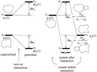
Notice that with the case 1 assumptions the energies after the interaction are raised and lowered by equal amounts, hAB, relative to the ``unperturbed'' energy, eA…ˆeB†, and the resulting wave functions are an equal admixture of the unperturbed wave functions.

Case 2: eA FeB , SAB I0, SAB f 1

This is a more realistic case since, if the two orbitals can interact, the overlap will not be zero. However, the overlap may be very small if the two orbitals are far apart, and in this case, a mathematical simpli®cation ensues, as seen below.

When the overlap is not zero (assumed positive), the solutions may again conveniently

The second part of equations (3.24) and (3.25) arises from the expansion of 1=…1 G SAB†, which converges rapidly if SAB f 1. Thus it is apparent that inclusion of the overlap term reduces the amount of stabilization of the bonding combination of orbitals as well as the amount of destabilization of the antibonding combination. However, the reduction of the amount of destabilization, j…eA ÿ hAB†SABj, is less than the reduction in the amount of stabilization, j…eA ‡ hAB†SABj, leaving the antibonding combination somewhat higher in energy than the bonding combination relative to the reference unperturbed energy. The situation is illustrated in Figure 3.2. This last result, which is a consequence of overlap, is fundamental to the application of orbital interaction theory. The precise amount of destabilization for the degenerate case may be calculated by

De ˆ eU ‡ eL ÿ 2eA

The energy change after interaction depends on two terms according to equation (3.26). The ®rst term, involving ÿhABSAB, is positive and contributes to the destabilization. The second term, which is proportional to the energy of the interacting orbitals, is negative since eA…ˆhAA† is negative and leads to a stabilization. The ®rst term is expected to dominate since SAB < 1, and for valence orbitals, the intrinsic interaction energy, hAB, is of the same order of magnitude (though smaller) as the orbital energy, eA. We will return to this point in our case 4 study.

It can be easily veri®ed by insertion of the precise value of eL and eU, equations (3.25) and (3.24), respectively, that the orbitals fL…1† and fU…1† again involve an equal

40 ORBITAL INTERACTION THEORY

Figure 3.2. Case 2: (a) Perturbation view of interaction of two orbitals with inclusion of overlap; (b) standard interaction diagram showing relative destabilization of the upper orbital.

admixture of the wA…1† and wB…1† in phase and out of phase, respectively, as in case 1, but the coe½cients are slightly di¨erent, namely

Case 3: eA IeB , SAB F0

For this case study, we again adopt the ``zero-overlap'' approximation but consider the nondegenerate case, assuming that eA > eB. The secular equation, from equation (3.15), becomes

If 4hAB2 f …eA ÿ eB†2, that is, the interaction energy is much less than the energy di¨er-

ence between the interacting orbitals, one can simplify equation (3.30) by expansion of the square root:

Notice that this situation is really only valid for separated systems. If the two orbitals are spatially close, say in the same molecule, it is unlikely that the last approximation would be appropriate. This situation is discussed further below.

In equation (3.31), the lower root is obtained by taking the minus sign. Thus

or

h2

eL A eB ÿ AB …3:33†

eA ÿ eB

Similarly,

Evidently, if the unperturbed orbitals are not of the same energy, and if the energy difference is large compared to the interaction energy, the e¨ect of the interaction is to lower the lower orbital further by an amount proportional to the square of the interaction energy and inversely proportional to the energy di¨erence. The upper orbital is raised by the same amount. One should suspect, correctly, that if overlap were to be taken into account, the amount of raising would be greater than the amount of lowering. Substitution of equations (3.33) and (3.34) separately into equations (3.11) and (3.12) yields the molecular orbitals. Speci®cally, insertion of equation (3.33) into equation (3.12), with SAB ˆ 0, yields

from which

42 ORBITAL INTERACTION THEORY

Figure 3.3. Case 3: (a) Perturbation view of interaction of two orbitals of unequal energy; (b) standard interaction diagram.

The factors cBL and cAU are determined by normalization, but this is not important for our purposes. Notice that the factor hAB=…eA ÿ eB† is negative and much less than 1 in absolute magnitude. Thus the lower MO is derived from the interacting orbital which has lower energy by the admixture of a small amount of the interacting orbital of higher energy. The signs of the coe½cients of the two interacting orbitals are the same, that is, ÿhAB=…eA ÿ eB† > 0. The upper MO is derived from the interacting orbital which has higher energy by the admixture of a small amount of the interacting orbital of lower energy. The signs of the coe½cients of the two interacting orbitals in the antibonding MO are di¨erent. (Note: The assertion about the relative signs of the coe½cients is contingent on the fact that the overlap of the two orbitals is positive.) The results from the case 3 study are depicted in Figure 3.3. Some of the results obtained above have been reviewed and applied by Ho¨mann in an investigation of orbital interactions through space and through bonds [6] and are used extensively in the excellent book by Albright et al. [58].

Case 4: eA IeB , SAB I0

As stated earlier, the exact algebraic solution of equation (3.15) is readily obtained but does not add to the concepts already derived. The orbital energies and wave functions

will resemble equations (3.33), (3.34) and (3.38), (3.39), respectively. The consequences of nonzero overlap will again prove to be that jDeUj > jDeLj. The dependence of the net destabilization, jDeUj ÿ jDeLj, was discussed in the case 2 study [equation (3.26)] and found to depend on two terms, a dominant destabilizing term and a stabilizing term which is proportional to the energy of the degenerate pair. The more general expression is easily derived. The roots of equation (3.15) by the quadratic formula are

As in the case 2 study, two terms of opposite sign are involved. The sum of orbital energies before and after interaction is the same when the quantity in square brackets [equation (3.42)] is zero, that is,

Equation (3.43) resembles the formula [equation (3.44)] adopted by Wolfsberg and Helmholtz [59] for the interaction matrix elements. This form, with the empirical factor k ˆ 1:75, was adopted by Ho¨mann in his derivation of extended HuÈckel theory [60], namely

That k should be between 1 and 2, and consequently that the sum of orbital energies after interaction should be greater than before the interaction, was o¨ered theoretical justi®cation by Woolley [61]. Substitution of (3.44) into (3.42) yields the result

In summary, at least for the frontier orbitals where equation (3.45) is expected to be valid, a net destabilization depending in a complex manner on the square of the overlap integral and proportional to the sum of unperturbed orbital energies ensues from the interaction.

44 ORBITAL INTERACTION THEORY

EFFECT OF OVERLAP

The magnitude of the overlap of the interacting orbitals has an in¯uence on the appearance of the interaction diagram because it a¨ects the magnitude of the interaction integral [equation (3.44)], the di¨erence between stabilization and destabilization [equation (3.45)], and the polarization of the resulting molecular orbitals, fL and fU. It is convenient to categorize the overlap dependence into two broad regimes, the regime of large overlap, which is usually the case when the interactions of interest are between adjacent regions of the same molecule (i.e., intramolecular), and the limit of small overlap, which is almost always the case when one is considering intermolecular interactions.

ENERGETIC EFFECT OF OVERLAP

Three kinds of energetic consequences must be considered: (a) the magnitudes of DeU and DeL, (b) the magnitude of the di¨erence between DeU and DeL; and (c) the dependence in the di¨erence in unperturbed orbital energies.

(a)The magnitudes of DeU and DeL are directly related to the magnitude of hAB; the larger the overlap, the larger is hAB, and the larger are DeU and DeL. Thus the energy changes which ensue from intramolecular interactions are usually much larger than those which originate intermolecularly.

(b)The relative magnitudes of DeU and DeL are directly related to the magnitude of the overlap as seen in equation (3.45); the larger the overlap, the larger is di¨erence between destabilization and stabilization. These considerations are important if both types (bonding and antibonding) of orbitals have to be occupied. Again, the individual energy changes which ensue from intramolecular interactions are usually much larger than those which originate intermolecularly.

(c)Larger overlap also means that it is more di½cult to meet the criterion for

the results displayed in equations (3.33) and (3.34), namely that the ratio jhAB=…eA ÿ eB†j is much less than unity. In other words, DeU and DeL are more closely proportional to hAB rather than its square and will not exhibit the inverse dependence on the di¨erence of the initial orbital energies. For intramolecular considerations, the orbital energy di¨erence becomes less important than the magnitude of hAB itself whereas for intermolecular interactions, orbital energy di¨erences are more important, and the inverse dependence on the energy di¨erence is expected.

ORBITAL EFFECT OF OVERLAP

The polarization of the resulting orbitals is also a¨ected by the overlap, although this is more di½cult to demonstrate algebraically and we do not do so here. We simply state the results: For a given energy di¨erence (not equal to zero), the larger the overlap, the less the polarization of fL and fU. Less polarization means greater mixing of the initial orbitals.

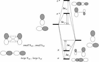
Figure 3.4. An s- and p-type interaction between p orbitals: The s orbitals are further apart and less polarized than the p orbitals. Also, jDes ÿ Desj > jDep ÿ Depj.

FIRST LOOK AT BONDING

A distinction between s and p orbitals may be made on the basis of the above considerations. Since the overlap of two p orbitals in a p fashion is smaller than in a s fashion, the p and p orbitals are closer together than the s and s orbitals because the smaller overlap results in smaller DeU and DeL. The s orbital is more antibonding relative to the s orbital than the p orbital is relative to the p orbital. Because of the smaller p-type overlap, one expects more polarization in the p orbitals than in the s orbitals. All three consequences are depicted in Figure 3.4.

RELATIONSHIP TO PERTURBATION THEORY

It should be apparent that the expressions for the wave functions after interaction [equations (3.38) and (3.39)] are equivalent to the Rayleigh±SchroÈdinger perturbation theory (RSPT) result for the perturbed wave function correct to ®rst order [equation (A.109)]. Similarly, the parallel between the MO energies [equations (3.33) and (3.34)] and the RSPT energy correct to second order [equation (A.110)] is obvious. The ``missing'' ®rst-order correction emphasizes the correspondence of the ®rst-order corrected wave function and the second-order corrected energy. Note that equations (3.33), (3.34), (3.38), and (3.39) are valid under the same conditions required for the application of perturbation theory, namely that the perturbation be weak compared to energy di¨erences.

46 ORBITAL INTERACTION THEORY

GENERALIZATIONS FOR INTERMOLECULAR INTERACTIONS

Equations (3.33), (3.34), (3.38), and (3.39) are valid under the condition that the perturbation be weak compared to energy di¨erences, that is, jhAB=…eA ÿ eB†j f 1. The case 1 and case 2 studies revealed the situation in the degenerate case. We now interpolate the intermediate situation, remembering that overlap will not be zero except when dictated to be so by local symmetry. However, overlap will always be small when dealing with interactions between molecules. Refer to Figures 3.1±3.4 for the de®ned quantities.

Generalization 1: DeL A DeU. The destabilization of the upper MO relative to the higher energy interacting orbital is approximately the same as the stabilization of the lower MO relative to the lower energy interacting orbital.

Generalization 2: jDeLjHjDeUj. The destabilization of the upper MO relative to the higher energy interacting orbital is always greater than the stabilization of the lower MO relative to the lower energy interacting orbital. This is a direct consequence of nonzero overlap [see equation (3.45)].

Generalization 3: (jDeUjCjDeLj) HjDeLj, jDeUj. The magnitude of the di¨erence between destabilization and stabilization is small compared to the actual magnitudes of the stabilization and destabilization.

Generalization 4: hAB (k a Positive Constant, SAB Assumed Positive). The interaction matrix element is not precisely proportional to the overlap integral but the behavior with respect to distance and symmetry is essentially the same. In other words, hAB will be zero by symmetry when SAB is zero by symmetry, but not otherwise. Also, hAB decreases in magnitude as a function of increasing separation in much the same way as SAB. Thus, two orbitals will not interact if they behave di¨erently toward local elements of symmetry.

The proportionality to the sum of unperturbed orbital energies [see also equation (3.44)] may be misleading. Large negative values for orbital energies are associated with core orbitals for which the overlap is close to zero.

Generalization 5: DeL A DeU A hAB2 =(eA CeB ). The energy raising and lowering depend directly on the square of the interaction matrix element (the square of the overlap matrix element) and inversely on the energy separation of the interacting orbitals. This relationship is precisely true only in the limit of very small interaction. The energy raising and lowering are maximum when the energy di¨erence is zero, in which case they have the value approximately hAB.

Generalization 6: j L A cB BdcA; j U A cA CdcB ; d FChAB /(eA CeB ); 0 Hd H1. The lower MO is polarized toward the lower interacting orbital and is the

in-phase (bonding) combination of the two. The upper MO is polarized toward the higher interacting orbital and is the out-of-phase (antibonding) combination of the two. In the limit of weak interaction, the amount of mixing of the minor component is approximately proportional to the interaction matrix element and inversely proportional to the energy di¨erence between the two interacting orbitals. The orbitals mix equally …d ˆ 1† when the orbital energy di¨erence is zero.

The above generalizations are summarized in Figure 3.5.

Figure 3.5. Orbital interaction diagrams: (a) nondegenerate case; (b) degenerate case.

ENERGY AND CHARGE DISTRIBUTION CHANGES FROM ORBITAL INTERACTION

The energy change which takes place upon the mixing of two orbitals depends on the number and distribution of the electrons. If neither orbital is occupied, there is no energy change. There is no need to calculate energy changes quantitatively. Inspection of the orbital interaction diagrams will provide the qualitative assessment of the energy change, that is, large or small, stabilizing or destabilizing. We consider separately the situations which may arise as a function of the number of electrons.

Four-Electron, Two-Orbital Interaction

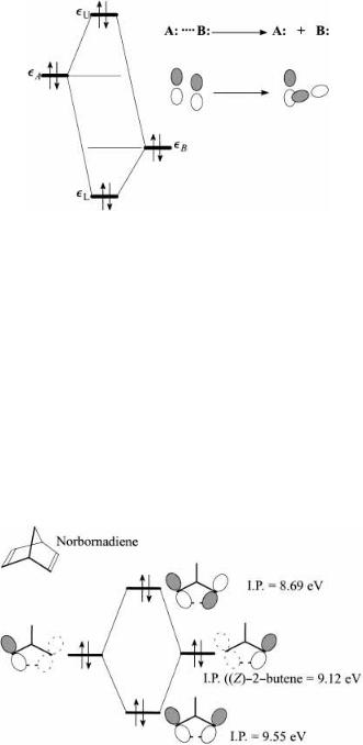
With four electrons, the bonding and antibonding molecular orbitals are both ®lled (Figure 3.6). The interaction will be repulsive and the system will adjust in such a way as to minimize the interaction. Closed-shell molecules will tend to repel each other. The common term is steric interaction. The net interactions between ®lled orbitals of two molecules separated by more than the van der Waals contact distance will be weak; the bonding and antibonding interactions, which may individually be large, almost cancel.

Filled orbitals which cannot physically separate because they are part of the same molecule may have substantially larger overlap than the intermolecular case, and the destabilizing interaction, DeU, may be much larger than the stabilizing interaction, DeL. The net repulsion will lead to conformational changes so as to minimize the repulsive interactions. If the interaction cannot be avoided by conformational change, then as the result of the interaction, a pair of electrons is raised in energy. The system has a lower

48 ORBITAL INTERACTION THEORY

Figure 3.6. Repulsive four-electron, two-orbital interaction: Closed-shell species will separate, ®lled orbitals will tend to align in each other's nodes.

ionization potential, is more easily oxidized, and is more basic in the Lewis sense. All of these features are observed in the experimental properties of norbornadiene (Figure 3.7). The inand out-of-phase interactions of the two occupied p bonding orbitals may be described by an interaction diagram such as shown in Figure 3.5b. Norbornadiene has two ionization potentials, 9.55 and 8.69 eV [62], which are above and below the ionization potential of …Z†-2-butene (9.12 eV [63]), cyclohexene (9.11 eV [64]), or norbornene (8.95 eV [64]), as expected on the basis of the orbital interaction diagram in Figure 3.7. The consequences of intramolecular interaction of s bonding orbitals is further discussed in Chapter 4.

Three-Electron, Two-Orbital Interaction

With three electrons one is dealing with a free radical. The bonding MO is doubly occupied and the antibonding molecular orbital has a single electron (Figure 3.8). In the

Figure 3.7. Four-electron, two-orbital interaction diagram for norbornadiene and its ionization potentials.