

Enzymes (Second Edition)
.pdf310 TIGHT BINDING INHIBITORS
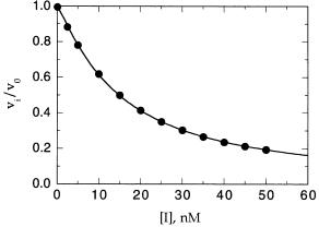
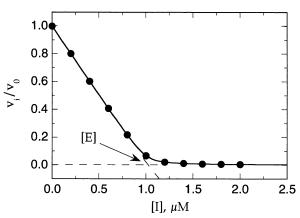
Figure 9.4 (A) Determination of ‘‘K’’ by the graphical method of Dixon (1972): dashed lines connect the starting point (v /v 1, [I] 0) with points on the curve where v /v v /n (n 2, 3, 4, and 5). Additional lines are drawn for apparent n 1 and apparent n 0, based on the x-axis spacing value ‘‘K,’’ determine from the n 2—5 lines (see text for further details). (B) Secondary plot of the ‘‘K ’’ as a function of substrate concentration for a tight binding competitive inhibitor. Graphical determinations of K and K are obtained from the values of the y and x intercepts of the plot, respectively, as shown.
Knowing the value of K from a nest of these lines, one can draw additional lines from the x axis to the origin at spacing of K on the x axis, for apparent values of n 1 and n 0. From this treatment, the line corresponding to n 0 will intersect the x axis at a displacement from the origin that is equal to the total enzyme concentration, [E]. Dixon goes on to show that in the case of a noncompetitive inhibitor ( 1), the spacing value K is equal to the inhibitor K , and a plot of K as a function of substrate concentration will be a horizontal line; that is, the value of K for a noncompetitive inhibitor is independent of substrate concentration. For a competitive inhibitor, however, the measured value of K will increase with increasing substrate concentration. A replot of K as a function of substrate concentration yields estimates of the K of the inhibitor and the K of the substrate from the y and x intercepts, respectively (Figure 9.4B).
9.3 DETERMINING Ki FOR TIGHT BINDING INHIBITORS
The literature describes several methods for determining the K value of a tight binding enzyme inhibitor. We have already discussed the graphical method of Dixon (1972), which allows one to simultaneously distinguish inhibitor type and calculate the K . A more mathematical treatment of tight binding inhibitors, presented by Morrison (1969), led to a generalized equation to describe the fractional velocity of an enzymatic reaction as a function of inhibitor concentration, at fixed concentrations of enzyme and substrate. This equation, commonly referred to as the Morrison equation, is derived in a manner similar to Equation 4.38, except that here the equation is cast in terms of fractional enzymatic activity in the presence of the inhibitor (i.e., in terms of the fraction

DETERMINING Ki FOR TIGHT BINDING INHIBITORS |
311 |
of free enzyme instead of the fraction of inhibitor-bound enzyme).
v |
|
|
([E] [I] K ) |
([E] [I] K ) 4[E][I] |
|
||
|
1 |
|
|
|
(9.6) |
||
v |
|
|
2[E] |
|
|
||
|
|
|
|
|
|
|
|
The form of K in Equation 9.6 varies with inhibitor type. The following explicit forms of this parameter for the different inhibitor types are similar to those presented in Equations 9.2—9.5 for the IC values.
For competitive inhibitors:
K |
K 1 |
[S] |
|
|||||||
K |
||||||||||
|
|
|
|
|
||||||
|
|
|
|
|
||||||
For Noncompetitive Inhibitors: |
|
|
|
|
|
|
||||
K |
[S] K |
|
|
|||||||
|
|
K |
|
[S] |
|
|||||
|
|
|
||||||||
|
|
K |
|
K |
|
|
||||
|
|
|
|
|
|
|
||||
when 1: |
|
|
|
|
|
|
|
|
|
|
|
K K |
|
|
|
|
|
||||
|
|
|
|
|
|
|
|
|||
For uncompetitive inhibitors: |
|
|
|
|
|
|
|
|
|
|
|
K 1 |
|
K |
|
||||||
K |
|
[S] |
||||||||
(9.7)
(9.8)
(9.9)
(9.10)
Prior to the widespread use of computer-based routines for curve fitting, the direct use of the Morrison equation was inconvenient for extracting inhibitor constants from experimental data. To overcome this limitation, Henderson (1972) presented the derivation of a linearized form of the Morrison equation that allowed graphical determination of K and [E] from measurements of the fractional velocity as a function of inhibitor concentration at a fixed substrate concentration. The generalized form of the Henderson equation is as follows:
|
v |
|
v |
|
|
|
|
[I] |
K |
v |
|
[E] |
(9.11) |
||
|
|
|
|||||
1 |
|
|
|
|
|
|
|
|
|
|
|
|
|
|
|
v |
|
|
|
|
|
|
|
where K has the same forms as presented in Equations 9.7—9.10 for the various inhibitor types.
Inspection reveals that Equation 9.11 is a linear equation. Hence, if one were to plot [I]/(1 v /v ) as a function of v /v (i.e., the reciprocal of the fractional

312 TIGHT BINDING INHIBITORS
Figure 9.5 Henderson plot for a tight binding inhibitor.
velocity), the data could be fit to a straight line with slope equal to K and y intercept equal to [E], as illustrated in Figure 9.5. Note that the Henderson method yields a straight-line plot regardless of the inhibitor type. The slope of the lines for such plots will, however, vary with substrate concentration in different ways depending on the inhibitor type. The variation observed is similar to that presented in Figure 9.3 for the variation in IC value for different tight binding inhibitors as a function of substrate concentration. Thus, the Henderson plots also can be used to distinguish among the varying inhibitor binding mechanisms.
While linearized Henderson plots are convenient in the absence of a computer curve-fitting program, the data treatment does introduce some degree of systematic error (see Henderson, 1973, for a discussion of the statistical treatment of such data). Today, with the availability of robust curve-fitting routines on laboratory computers, it is no longer necessary to resort to linearized treatments of data such as the Henderson plots. The direct fitting of fraction velocity versus inhibitor concentration data to the Morrison equation (Equation 9.6) is thus much more desirable, and is strongly recommended.
Figure 9.6 illustrates the direct fitting of fractional velocity versus inhibitor concentration data to Equation 9.6. Such data would call for predetermination of the K value for the substrate (as described in Chapter 5) and knowledge of the substrate concentration in the assays. Then the data, such as the points in Figure 9.6, would be fit to the Morrison equation, allowing both K and [E] to be simultaneously determined as fitting parameters. Measurements of this type at several different substrate concentrations would allow determination of the mode of inhibition, and thus the experimentally measured K
values could be converted to true K values.
In the case of competitive tight binding inhibitors, an alternative method for determining inhibitor K is to measure the iniital velocity under conditions of
USE OF TIGHT BINDING INHIBITORS |
313 |
Figure 9.6 Plot of fractional velocity as a function of inhibitor concentration for a tight binding inhibitor. The solid curve drawn through the data points represents the best fit to the Morrison equation (Equation 9.6).
extremely high substrate concentration (Tornheim, 1994). Reflecting on Equation 9.2, we see that if the ratio [S]/K is very large, the IC will be much greater than the enzyme concentration, even though the K is similar in magnitude to [E]. Thus, if a high enough substrate concentration can be experimentally achieved, the tight binding nature of the inhibitor can be overcome, and the K can be determined from the measured IC by application of a rearranged form of Equation 9.2. Tornheim recommends adjusting [S] so that the ratios [S]/K and [I]/K are about equal for these measurements. Not all enzymatic reactions are amenable to this approach, however, because of the experimental limitations on substrate concentration imposed by the solubility of the substrate and the analyst’s ability to measure a linear initial velocity under such extreme conditions. In favorable cases, however, this approach can be used with excellent results.
9.4 USE OF TIGHT BINDING INHIBITORS TO DETERMINE ACTIVE ENZYME CONCENTRATION
In many experimental strategies one wishes to know the concentration of enzyme in a sample for subsequent data analysis. This approach applies not only to kinetic data, but also to other types of biochemical and biophysical studies with enzymes. The literature gives numerous methods for determining total protein concentration in a sample, on the basis of spectroscopic, colorimetric, and other analytical techniques (see Copeland, 1994, for some examples). All these methods, however, measure bulk protein concentration rather than the concentration of the target enzyme in particular. Also, these
314 TIGHT BINDING INHIBITORS
Figure 9.7 Determination of active enzyme concentration by titration with a tight binding inhibitor. [E] 1.0 M, K 5 nM (i.e., [E]/K 200). The solid curve drawn through the data is the best fit to the Morrison equation (Equation 9.6). The dashed lines were drawn by linear least-squares fits of the data at inhibitor concentrations that were low (0—0.6 M) and high
(1.4—2.0 M), respectively. The active enzyme concentration is determined from the x-axis value at the intersection of the two straight lines.
methods do not necessarily distinguish between active enzyme molecules, and molecules of denatured enzyme. In many of the applications one is likely to encounter, it is the concentration of active enzyme molecules that is most relevant. The availability of a tight binding inhibitor of the target enzyme provides a convenient means of accurately determining the concentration of active enzyme in the sample, even in the presence of denatured enzyme or other nonenzymatic proteins.
Referring back to Equation 9.6, if we set up an experiment in which both [E] and [I] are much greater than K , we can largely ignore the K term in this equation. Under these conditions, the fractional velocity of the enzymatic reaction will fall off quasi-linearly with increasing inhibitor concentration until [I] [E]. At this point the fractional velocity will approach zero and remain there at higher inhibitor concentrations. In this case, a plot of fractional velocity as a function of inhibitor concentration will look like Figure 9.7 when fit to the Morrison equation. The data in figure 9.7 were generated for a hypothetical situation: K of inhibitor, 5 nM; active enzyme concentration of the sample, 1.0 M (i.e., [E]/K 200). The data at lower inhibitor concentration can be fit to a straight line that is extended to the x axis (dashed line in Figure 9.7), and the data points at higher inhibitor concentrations can be fit to a straight horizontal line at v /v 0 (longer dashed line in Figure 9.7). The two lines thus drawn will intersect at a point on the x axis where [I] [E]. Note, however, that this treatment works only when [E] is much greater than K . When [E] is less than about 200K , the data are not well described by two
SUMMARY 315
intersecting straight lines. In such cases the data can be fit directly to Equation 9.6 to determine [E], as described earlier.
This type of treatment is quite convenient for determining the active enzyme concentration of a stock enzyme solution (i.e., at high enzyme concentration) that will be diluted into a final reaction mixture for experimentation. For example, one might wish to store an enzyme sample at a nominal enzyme concentration of 100 M in a solution containing 1 mg/mL gelatin for stability purposes (see discussion in Chapter 7). The presence of the gelatin would preclude accurate determination of enzyme concentration by one of the traditional colorimetric protein assays; moreover, active enzyme concentration could not be determined by means of such assays. Given a nanomolar inhibitor of the target enzyme, one could dilute a sample of the stock enzyme to some convenient concentration for an enzymatic assay that was still much greater than the K (e.g., 1 M). Treatment of the fractional velocity versus inhibitor concentration as described here would thus lead to determination of the true concentration of active enzyme in the working solution, and from this one could back-calculate to arrive at the true concentration of active enzyme in the enzyme stock. This is a routine strategy in many enzymology laboratories, and numerous examples of its application can be found in the literature.
A comparable assessment of active enzyme concentration can be obtained by the reverse experiment in which the inhibitor concentration is fixed at some value much greater than the K (about 200 K or more), and the amount of enzyme added to the reaction mixture is varied. The results of such an experiment are illustrated in Figure 9.8. The initial velocity remains zero until equal concentrations of enzyme and inhibitor are present in solution. As the enzyme concentration is titrated beyond this point, the stoichiometric inhibition is overcome, and a linear increase in initial velocity is then observed. Again, from the point of intersection of the two dashed lines drawn through the data as in Figure 9.8, the true concentration of active enzyme can be determined (Williams and Morrison, 1979). An advantage of this second approach to active enzyme concentration determination is that it typically uses up less of the enzyme stock to complete the titration. Hence, when the enzyme is in limited supply, this alternative is recommended.
9.5 SUMMARY
In this Chapter we have described a special case of enzyme inhibition, in which the dissociation constant of the inhibitor is similar to the total concentration of enzyme in the sample. These inhibitor offer a special challenge to the enzymologist, because they cannot be analyzed by the traditional methods described in Chapter 8. We have seen that tight binding inhibitors yield double-reciprocal plots that appear to suggest noncompetitive inhibition regardless of the true mode of interaction between the enzyme and the inhibitor. Thus, whenever noncompetitive inhibition is diagnosed through the use of double reciprocal

316 TIGHT BINDING INHIBITORS
Figure 9.8 Determination of active enzyme concentration by titration of a fixed concentration of a tight binding inhibitor with enzyme: [I] 200 nM, K 1 nM (i.e., [I]/K 200). The data analysis is similar to that described for Figure 9.7 and in the text. Velocity is in arbitrary units.
plots, the data should be reevaluated to ensure that tight binding inhibition is not occurring. Methods for determining the true mode of inhibition and the K for these tight binding inhibitors were described in this chapter.
Tight binding inhibitors are an important class of molecules in many industrial enzyme applications. Many contemporary therapeutic enzyme inhibitors, for example, act as tight binders. Recent examples include inhibitors of dihydrofolate reductase (as anticancer drugs), inhibitors of the HIV aspartyl protease, (as anti-AIDS drugs), and inhibitors of metalloproteases (as potential cartilage protectants). Many of the naturally occurring enzyme inhibitors, which play a role in metabolic homeostasis, are tight binding inhibitors of their target enzymes. Thus tight binding inhibitors are an important and commonly encountered class of enzyme inhibitor. The need for special treatment of enzyme kinetics in the presence of these inhibitors must not be overlooked.
REFERENCES AND FURTHER READING
Bieth, J. (1974) In Proteinase Inhibitors, Bayer-Symposium V, Springer-Verlag, New York, pp. 463—469.
Cha, S. (1975) Biochem. Pharmacol. 24, 2177.
Cha, S. (1976) Biochem. Pharmacol. 25, 2695.
Cha, S., Agarwal, R. P., and Parks, R. E., Jr. (1975) Biochem. Pharmacol. 24, 2187. Copeland, R. A. (1994) Methods of Protein Analysis, A Practical Guide to L aboratory
Protocols, Chapman & Hall, New York.
Copeland, R. A., Lombardo, D., Giannaras, J., and DeCicco, C. P. (1995) Bioorg. Med. Chem. L ett. 5, 1947.
REFERENCES AND FURTHER READING |
317 |
Dixon, M. (1972) Biochem. J. 129, 197.
Dixon, M., and Webb, E. C. (1979) Enzymes, 3rd ed., Academic Press, New York. Goldstein, A. (1944) J. Gen. Physiol. 27, 529.
Greco, W. R., and Hakala, M. T. (1979) J. Biol. Chem. 254, 12104. Henderson, P. J. F. (1972) Biochem. J. 127, 321.
Henderson, P. J. F. (1973) Biochem. J. 135, 101.
Morrison, J. F. (1969) Biochim. Biophys. Acta, 185, 269.
Myers, D. K. (1952) Biochem. J. 51, 303.
Szedlacsek, S. E., and Duggleby, R. G. (1995) Methods Enzymol. 249, 144. Tornheim, K. (1994) Anal. Biochem. 221, 53.
Turner, P. M., Lerea, K. M., and Kull, F. J. (1983) Biochem. Biophys. Res. Commun. 114, 1154.
Williams, J. W., and Morrison, J. F. (1979) Methods Enzymol. 63, 437.
Williams, J. W., Morrison, J. F., and Duggleby, R. G. (1979) Biochemistry, 18, 2567.
Enzymes: A Practical Introduction to Structure, Mechanism, and Data Analysis.
Robert A. Copeland Copyright 2000 by Wiley-VCH, Inc.
ISBNs: 0-471-35929-7 (Hardback); 0-471-22063-9 (Electronic)
10
TIME-DEPENDENT
INHIBITION
All the inhibitors we have encountered thus far have established their binding equilibrium with the enzyme on a time scale that is rapid with respect to the turnover rate of the enzyme-catalyzed reaction. In Chapter 9 we noted that many tight binding inhibitors establish this equilibrium on a slower time scale, but in our discussion we eliminated this complication by pretreating the enzyme with the inhibitor long enough to ensure that equilibrium had been fully reached before steady state turnover was initiated by addition of substrate. In this chapter we shall explicitly deal with inhibitors that bind slowly to the enzyme on the time scale of enzymatic turnover, and thus display a change in initial velocity with time. These inhibitors, that is, act as slow binding or time-dependent inhibitors of the enzyme.
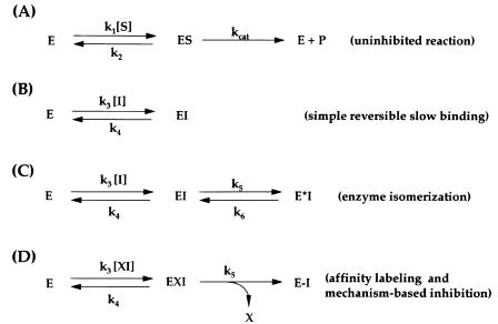
We can distinguish four different modes of interaction between an inhibitor and an enzyme that would result in slow binding kinetics. The equilibria involved in these processes are represented in Figure 10.1. Figure 10.1A shows the equilibrium associated with the uninhibited turnover of the enzyme, as we discussed in Chapter 5: k , the rate constant associated with substrate binding to the enzyme to form the ES complex, is sometimes refered to as k (for substrate coming on to the enzyme). The constant k in Figure 10.1A is the dissociation or off rate constant for the ES complex dissociating back to free enzyme and free substrate, and k is the catalytic rate constant as defined in Chapter 5.
In the remaining schemes of Figure 10.1 (B—D), the equilibrium described by Scheme A occurs as a competing reaction (as we saw in connection with simple reversible enzyme inhibitors in Chapter 8).
Scheme B illustrates the case of the inhibitor binding to the enzyme in a simple bimolecular reaction, similar to what we discussed in Chapters 8 and 9.
318
TIME-DEPENDENT INHIBITION |
319 |
Figure 10.1 Schemes for time-dependent enzyme inhibition. Scheme A, which describes the turnover of the enzyme in the absence of inhibitor, is a competing reaction for all the other schemes. Scheme B illustrates the equilibrium for a simple reversible inhibition process that leads to time-dependent inhibition because of the low values of k and k relative to enzyme turnover. In Scheme C, an initial binding of the inhibitor to the enzyme leads to formation of the
EI complex, which undergoes an isomerization of the enzyme to form the new complex E*I.
Scheme D represents the reactions associated with irreversible enzyme inactivation due to covalent bond formation between the enzyme and some reactive group on the inhibitor, leading to the covalent adduct E—I. Inhibitors that conform to Scheme D may act as affinity labels of the enzyme, or they may be mechanism-based inhibitors.
Here, however, the association and dissociation rate constants (k and k , respectively) are such that the equilibrium is established slowly. As with rapid binding inhibitors, the equilibrium dissociation constant K is given here by:
|
k |
|
[E][I] |
||
K |
|
|
|
|
(10.1) |
k |
|
||||
|
|
[EI] |
|||
Morrison and Walsh (1988) have pointed out that even when k is diffusion limited, if K is low and [I] is varied in the region of K , both k [I] and k will be low in value. Hence, under these circumstances onset of inhibition would be slow even though the magnitude of k is that expected for a rapid reaction. This is why most tight binding inhibitors display time-dependent inhibition. If the observed time dependence is due to an inherently slow rate of binding, the inhibitor is said to be a slow binding inhibitor, and its dissociation constant is given by Equation 10.1. If, on the other hand, the inhibitor is also a tight