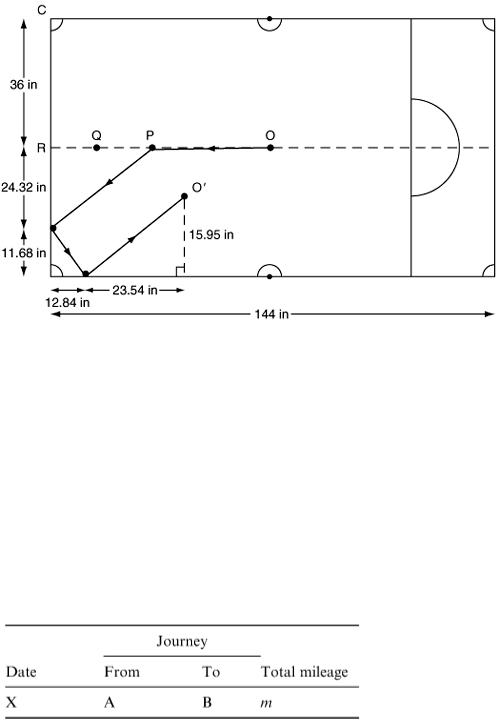
Figure 9.27

Can the black ball now be potted, and if so what must be the angle of aim for the cue ball? Further calculation shows that we should aim so as to cover half the black ball on impact, with again a very small margin of error. Snooker is a difficult game to play well!

9.12 Further models

We conclude with a selection of modelling exercises for you to try your skills on. They are not arranged in any particular order and some may be easier than others.

Mileage

Employees of a firm send in claims for travelling expenses which are paid according to the mileage which they have travelled during the course of their work. The claim form requires each person to fill in details as follows.

The clerk who processes the claims has been told to check the mileage figures using the map but she is very short of time and resorts to using a ruler and measuring the straight-line distance s from A to B. s is obviously an underestimate of m. Can you develop a mathematical model for estimating m from s: m = f(s) ?

Check your model by measuring a number of distances on a map and give an overall assessment of the accuracy of your model.

Is it better to use one formula for smaller distances, say up to 50 miles, and a different formula for longer distances?

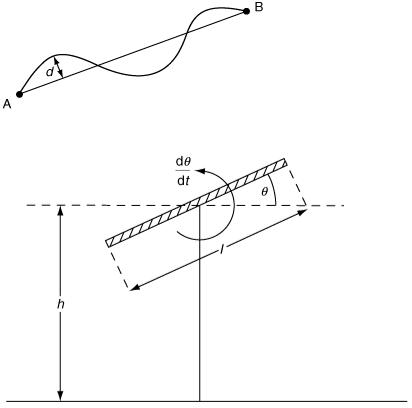
If the largest deviation d measured at right angles to AB is also measured can the value of d be incorporated into the model to improve the accuracy (Figure 9.28)?

Figure 9.28

Figure 9.29

Heads or tails

The result of tossing a coin is normally regarded as a random event with equal probabilities of heads and tails. In reality of course the outcome is entirely dependent on the initial conditions which set the coin in motion and, if these conditions and all the other relevant properties were known, we could predict the outcome.

Figure 9.29 illustrates a simple model in which the coin is represented by a straight-line segment of length l, held initially at an inclination θ to the horizontal and with its centre at height h above a horizontal table.

Suppose that the ‘coin’ is set spinning with angular speed dθ/d t and falls under gravity so that its centre moves along the vertical line shown in the sketch. Assume that the outcome is determined when one end or the other of the coin hits the table, i.e. do not try to model ‘bouncing’ off the table.

The objective is to discover how the outcome (heads or tails) depends on the values of h, l, θ and dθ/d t.

Picture hanging

A picture (modelled as a rectangle) is to be suspended from a hook on a vertical wall by means of a piece of string attached to the back of the picture at two points as shown in Figure 9.30.

The relevant parameters are the lengths a, b, c and d indicated in the sketch, the length l of the string and the coefficient of friction between the picture and the wall.

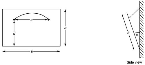
Figure 9.30

Develop a mathematical model which will enable you to find how the tension in the string depends on the other parameters, and in particular how to choose the length of the string and the points of attachment so that the string is least likely to break.

Also find the angle α of inclination.

For what range of values of the parameters will the string be visible above the top edge of the painting when viewed horizontally?

Motorway

A motorway is to be built between cities A and B. City B is 20 km due south and 30 km due east of city A and there is a range of mountains running approximately east–west which lies between them. The cost of motorway building is related to the nature of the terrain and in Figure 9.31 the whole area has been modelled in a very simple way using three different terrain types in parallel east–west strips.

Your task is to develop a mathematical model which will help to determine the cheapest route for the motorway given the relative costs per kilometre of construction for the three types of terrain and the widths of the strips. In the diagram the straight line route AB is obviously the shortest in distance but will not necessarily be the cheapest. A route such as ARSB has a short mountain section but is this the best solution? How would you adapt your model to incorporate the following two constraints.

1.When the route changes direction, the angle made must be at least 140°.

2.The route must pass through a given point such as P in order to merge with an existing road.

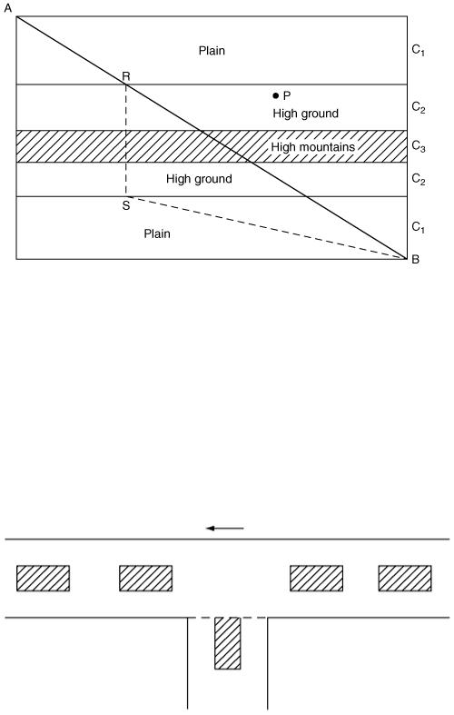
Figure 9.31

Vehicle-merging delay at a junction

Figure 9.32 shows a single-lane traffic stream on the major road and a minor approach road (no right turns allowed). The traffic flow rate on the major road is known, say q vehicles per hour. The time gaps (measured at a fixed point) between vehicles on the main road can be assumed to be independent random variables.

Assume that vehicles arrive at random times on the minor road and that a driver will merge with the stream of traffic on the main road if he finds a time gap sufficiently large for his safe entry. We can model this by assuming the driver will always reject time gaps less than some minimum time gap T and that merging only takes place for time gaps greater than T. The delay time of the driver is zero if an acceptable time gap is available at the instant that he arrives at the junction; otherwise the driver has to wait for an acceptable gap.

Figure 9.32

Make what you think are reasonable assumptions about the values of q and T and any other parameters involved in the model. Find the distribution of delay times at the junction and investigate how this distribution depends on the other parameters.