

Chapter 26Neural Networks (and more!) |
461 |
x1
x2
FIGURE 26-6
Neural network active node. This is a flow diagram of the active nodes used in the hidden and output layers of the neural network. Each input is multiplied by a weight (the wN values), and then summed. This produces a single value that is passed through an "s" shaped nonlinear function called a sigmoid. The sigmoid function is shown in more detail in Fig. 26-7.
x3 |
|
|
|
|
w1 |
|
|
|
|
|
|
|
|
|
|
|
|
|
|
|
|
|
|
|
|
|
|||
|
|
|
|
|
|
|
|
|
|
|
SUM |
|
SIGMOID |
||||||||||||||||
|
|
|
|
|
|
|
|
w2 |
|
|
|||||||||||||||||||
x4 |
w3 |
|
|||||||||||||||||||||||||||
|
|
|
|
|
|
|
|
|
|
|
|
|
|
|
|
|
|
|
|
|
|
|
|
||||||
|
|
|
|
|
|
|
|
|
|
|
E |
|
|
|
|
|
|
|
|
|
|
|
|
|
|
|
|
||
|
|
|
|
|
|
|
|
|
|
|
|
|
|
|
|
|
|
|
|
|
|
|
|
|
|
|
|||
x5 |
|
|
|
|
|
|
|
w4 |
|
|
|
|
|
|
|
|
|
|
|
|
|
|
|
|
|
|
|||
|
|
|
|
|
|
|
|
|
|
|
|
|
|
|
|
|
|||||||||||||
|
|
|
|
|
|
|
|
|
|
|
|
|
|
|
|
|
|
|
|
|
|
|
|||||||
|
w5 |
|
|
|
|
|
|
|
|
|
|
|
|
|
|
|
|
||||||||||||
|
|
|
|
|
|
|
|
|
|
|
|
|
|
|
|
||||||||||||||
|
|
|
w6 |
|
|
|
|
|
|
|
|
|
|
|
|
|
|
|
|
|
|||||||||
|
|
|
|
|
|
|
|
|
|
|
|
|
|
|
|
|
|
|
|
|
|
|
|
|
|||||
x6 |
|
|
|
|
|
|
|
|
|
|
|
|
|
|
|
|
|
|
|
|
|
|
|
|
|||||
|
|
|
|
|
|
|
|
|
|
|
|
|
|
|
|
|
|||||||||||||
|
|
|
|
|
|
|
|
|
|
|
|
|
|
|
|
|
|
|
|
|
|
||||||||
|
|
|
w7 |
|
|
|
|
|
|
|
|
|
|
|
|
|
|
|
|
|
|||||||||
WEIGHT
x7
With other weights, the outputs might classify the objects as: metal or nonmetal, biological or nonbiological, enemy or ally, etc. No algorithms, no rules, no procedures; only a relationship between the input and output dictated by the values of the weights selected.
100 |
'NEURAL NETWORK (FOR THE FLOW DIAGRAM IN FIG. 26-5) |
|
110 |
' |
|
120 |
DIM X1[15] |
'holds the input values |
130 |
DIM X2[4] |
'holds the values exiting the hidden layer |
140 |
DIM X3[2] |
'holds the values exiting the output layer |
150 |
DIM WH[4,15] |
'holds the hidden layer weights |
160 |
DIM WO[2,4] |
'holds the output layer weights |
170 |
' |
|
180 |
GOSUB XXXX |
'mythical subroutine to load X1[ ] with the input data |
190 |
GOSUB XXXX |
'mythical subroutine to load the weights, WH[ , ] & W0[ , ] |
200 |
' |
|
210 |
' |
'FIND THE HIDDEN NODE VALUES, X2[ ] |
220 FOR J% = 1 TO 4 |
'loop for each hidden layer node |
|
230 |
ACC = 0 |
'clear the accumulator variable, ACC |
240 |
FOR I% = 1 TO 15 |
'weight and sum each input node |
250 |
ACC = ACC + X1[I%] * WH[J%,I%] |
|
260 |
NEXT I% |
|
270 |
X2[J%] = 1 / (1 + EXP(-ACC) ) |
'pass summed value through the sigmoid |
280 NEXT J% |
|
|
290 |
' |
|
300 |
' |
'FIND THE OUTPUT NODE VALUES, X3[ ] |
310 FOR J% = 1 TO 2 |
'loop for each output layer node |
|
320 |
ACC = 0 |
'clear the accumulator variable, ACC |
330 |
FOR I% = 1 TO 4 |
'weight and sum each hidden node |
340 |
ACC = ACC + X2[I%] * WO[J%,I%] |
|
350 |
NEXT I% |
|
360 |
X3[J%] = 1 / (1 + EXP(-ACC) ) |
'pass summed value through the sigmoid |
370 NEXT J% |
|
|
380 |
' |
|
390 END |
TABLE 26-1 |
|
|
|
|
462 |
The Scientist and Engineer's Guide to Digital Signal Processing |
1.0 |
0.3 |
a. Sigmoid function |
b. First derivative |
0.8 |
|
|
0.2 |
0.6 |
s`(x) |
s(x) |
|
0.4 |
|
|
0.1 |
0.2 |
|
0.0 |
0.0 |
-7 -6 -5 -4 -3 -2 -1 0 1 2 3 4 5 6 7 |
-7 -6 -5 -4 -3 -2 -1 0 1 2 3 4 5 6 7 |
x |
x |
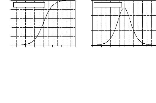
FIGURE 26-7 |
|
The sigmoid function and its derivative. Equations 26-1 and 26-2 generate these curves. |
|
Figure 26-7a shows a closer look at the sigmoid function, mathematically described by the equation:
EQUATION 26-1
The sigmoid function. This is used in neural networks as a smooth threshold. This function is graphed in Fig. 26-7a.
1
s (x) '
1% e & x
The exact shape of the sigmoid is not important, only that it is a smooth threshold. For comparison, a simple threshold produces a value of one when x > 0 , and a value of zero when x < 0 . The sigmoid performs this same basic thresholding function, but is also differentiable, as shown in Fig. 26-7b. While the derivative is not used in the flow diagram (Fig. 25-5), it is a critical part of finding the proper weights to use. More about this shortly. An advantage of the sigmoid is that there is a shortcut to calculating the value of its derivative:
EQUATION 26-2
First derivative of the sigmoid function. This is calculated by using the value of the sigmoid function itself.
s N(x) ' s (x) [ 1 & s (x) ]
For example, if x ' 0 , then s (x ) ' 0.5 (by Eq. 26-1), and the first derivative is calculated: s N(x ) ' 0.5 (1 & 0.5) ' 0.25 . This isn't a critical concept, just a trick to make the algebra shorter.
Wouldn't the neural network be more flexible if the sigmoid could be adjusted left-or-right, making it centered on some other value than x ' 0 ? The answer is yes, and most neural networks allow for this. It is very simple to implement; an additional node is added to the input layer, with its input always having a
Chapter 26Neural Networks (and more!) |
463 |
value of one. When this is multiplied by the weights of the hidden layer, it provides a bias (DC offset) to each sigmoid. This addition is called a bias node. It is treated the same as the other nodes, except for the constant input.
Can neural networks be made without a sigmoid or similar nonlinearity? To answer this, look at the three-layer network of Fig. 26-5. If the sigmoids were not present, the three layers would collapse into only two layers. In other words, the summations and weights of the hidden and output layers could be combined into a single layer, resulting in only a two-layer network.
Why Does It Work?
The weights required to make a neural network carry out a particular task are found by a learning algorithm, together with examples of how the system should operate. For instance, the examples in the sonar problem would be a database of several hundred (or more) of the 1000 sample segments. Some of the example segments would correspond to submarines, others to whales, others to random noise, etc. The learning algorithm uses these examples to calculate a set of weights appropriate for the task at hand. The term learning is widely used in the neural network field to describe this process; however, a better description might be: determining an optimized set of weights based on the statistics of the examples. Regardless of what the method is called, the resulting weights are virtually impossible for humans to understand. Patterns may be observable in some rare cases, but generally they appear to be random numbers. A neural network using these weights can be observed to have the proper input/output relationship, but why these particular weights work is quite baffling. This mystic quality of neural networks has caused many scientists and engineers to shy away from them. Remember all those science fiction movies of renegade computers taking over the earth?
In spite of this, it is common to hear neural network advocates make statements such as: "neural networks are well understood." To explore this claim, we will first show that it is possible to pick neural network weights through traditional DSP methods. Next, we will demonstrate that the learning algorithms provide better solutions than the traditional techniques. While this doesn't explain why a particular set of weights works, it does provide confidence in the method.
In the most sophisticated view, the neural network is a method of labeling the various regions in parameter space. For example, consider the sonar system neural network with 1000 inputs and a single output. With proper weight selection, the output will be near one if the input signal is an echo from a submarine, and near zero if the input is only noise. This forms a parameter hyperspace of 1000 dimensions. The neural network is a method of assigning a value to each location in this hyperspace. That is, the 1000 input values define a location in the hyperspace, while the output of the neural network provides the value at that location. A look-up table could perform this task perfectly, having an output value stored for each possible input address. The
464 |
The Scientist and Engineer's Guide to Digital Signal Processing |
difference is that the neural network calculates the value at each location (address), rather than the impossibly large task of storing each value. In fact, neural network architectures are often evaluated by how well they separate the hyperspace for a given number of weights.
This approach also provides a clue to the number of nodes required in the hidden layer. A parameter space of N dimensions requires N numbers to specify a location. Identifying a region in the hyperspace requires 2N values (i.e., a minimum and maximum value along each axis defines a hyperspace rectangular solid). For instance, these simple calculations would indicate that a neural network with 1000 inputs needs 2000 weights to identify one region of the hyperspace from another. In a fully interconnected network, this would require two hidden nodes. The number of regions needed depends on the particular problem, but can be expected to be far less than the number of dimensions in the parameter space. While this is only a crude approximation, it generally explains why most neural networks can operate with a hidden layer of 2% to 30% the size of the input layer.
A completely different way of understanding neural networks uses the DSP concept of correlation. As discussed in Chapter 7, correlation is the optimal way of detecting if a known pattern is contained within a signal. It is carried out by multiplying the signal with the pattern being looked for, and adding the products. The higher the sum, the more the signal resembles the pattern. Now, examine Fig. 26-5 and think of each hidden node as looking for a specific pattern in the input data. That is, each of the hidden nodes correlates the input data with the set of weights associated with that hidden node. If the pattern is present, the sum passed to the sigmoid will be large, otherwise it will be small.
The action of the sigmoid is quite interesting in this viewpoint. Look back at Fig. 26-1d and notice that the probability curve separating two bell shaped distributions resembles a sigmoid. If we were manually designing a neural network, we could make the output of each hidden node be the fractional probability that a specific pattern is present in the input data. The output layer repeats this operation, making the entire three-layer structure a correlation of correlations, a network that looks for patterns of patterns.
Conventional DSP is based on two techniques, convolution and Fourier analysis. It is reassuring that neural networks can carry out both these operations, plus much more. Imagine an N sample signal being filtered to produce another N sample signal. According to the output side view of convolution, each sample in the output signal is a weighted sum of samples from the input. Now, imagine a two-layer neural network with N nodes in each layer. The value produced by each output layer node is also a weighted sum of the input values. If each output layer node uses the same weights as all the other output nodes, the network will implement linear convolution. Likewise, the DFT can be calculated with a two layer neural network with N nodes in each layer. Each output layer node finds the amplitude of one frequency component. This is done by making the weights of each output layer node the same as the sinusoid being looked for. The resulting network correlates the
Chapter 26Neural Networks (and more!) |
465 |
input signal with each of the basis function sinusoids, thus calculating the DFT. Of course, a two-layer neural network is much less powerful than the standard three layer architecture. This means neural networks can carry out nonlinear as well as linear processing.
Suppose that one of these conventional DSP strategies is used to design the weights of a neural network. Can it be claimed that the network is optimal? Traditional DSP algorithms are usually based on assumptions about the characteristics of the input signal. For instance, Wiener filtering is optimal for maximizing the signal-to-noise ratio assuming the signal and noise spectra are both known; correlation is optimal for detecting targets assuming the noise is white; deconvolution counteracts an undesired convolution assuming the deconvolution kernel is the inverse of the original convolution kernel, etc. The problem is, scientist and engineer's seldom have a perfect knowledge of the input signals that will be encountered. While the underlying mathematics may be elegant, the overall performance is limited by how well the data are understood.
For instance, imagine testing a traditional DSP algorithm with actual input signals. Next, repeat the test with the algorithm changed slightly, say, by increasing one of the parameters by one percent. If the second test result is better than the first, the original algorithm is not optimized for the task at hand. Nearly all conventional DSP algorithms can be significantly improved by a trial-and-error evaluation of small changes to the algorithm's parameters and procedures. This is the strategy of the neural network.
Training the Neural Network
Neural network design can best be explained with an example. Figure 26-8 shows the problem we will attack, identifying individual letters in an image of text. This pattern recognition task has received much attention. It is easy enough that many approaches achieve partial success, but difficult enough that there are no perfect solutions. Many successful commercial products have been based on this problem, such as: reading the addresses on letters for postal routing, document entry into word processors, etc.
The first step in developing a neural network is to create a database of examples. For the text recognition problem, this is accomplished by printing the 26 capital letters: A,B,C,D þ Y,Z, 50 times on a sheet of paper. Next, these 1300 letters are converted into a digital image by using one of the many scanning devices available for personal computers. This large digital image is then divided into small images of 10×10 pixels, each containing a single letter. This information is stored as a 1.3 Megabyte database: 1300 images; 100 pixels per image; 8 bits per pixel. We will use the first 260 images in this database to train the neural network (i.e., determine the weights), and the remainder to test its performance. The database must also contain a way of identifying the letter contained in each image. For instance, an additional byte could be added to each 10×10 image, containing the letter's ASCII code. In another scheme, the position
466 |
The Scientist and Engineer's Guide to Digital Signal Processing |
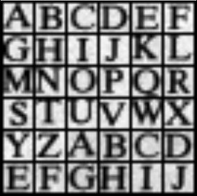
FIGURE 26-8
Example image of text. Identifying letters in images of text is one of the classic pattern recognition problems. In this example, each letter is contained in a 10×10 pixel image, with 256 gray levels per pixel. The database used to train and test the example neural network consists of 50 sets of the 26 capital letters, for a total of 1300 images. The images shown here are a portion of this database.
of each 10×10 image in the database could indicate what the letter is. For example, images 0 to 49 might all be an "A", images 50-99 might all be a "B", etc.
For this demonstration, the neural network will be designed for an arbitrary task: determine which of the 10×10 images contains a vowel, i.e., A, E, I, O, or U. This may not have any practical application, but it does illustrate the ability of the neural network to learn very abstract pattern recognition problems. By including ten examples of each letter in the training set, the network will (hopefully) learn the key features that distinguish the target from the nontarget images.
The neural network used in this example is the traditional three-layer, fully interconnected architecture, as shown in Figs. 26-5 and 26-6. There are 101 nodes in the input layer (100 pixel values plus a bias node), 10 nodes in the hidden layer, and 1 node in the output layer. When a 100 pixel image is applied to the input of the network, we want the output value to be close to one if a vowel is present, and near zero if a vowel is not present. Don't be worried that the input signal was acquired as a two-dimensional array (10×10), while the input to the neural network is a one-dimensional array. This is your understanding of how the pixel values are interrelated; the neural network will find relationships of its own.
Table 26-2 shows the main program for calculating the neural network weights, with Table 26-3 containing three subroutines called from the main program. The array elements: X1[1] through X1[100], hold the input layer values. In addition, X1[101] always holds a value of 1, providing the input to the bias node. The output values from the hidden nodes are contained
|
Chapter 26Neural Networks (and more!) |
467 |
|
100 |
'NEURAL NETWORK TRAINING (Determination of weights) |
|
|
110 |
' |
|
|
120 |
|
'INITIALIZE |
|
130 MU = .000005 |
'iteration step size |
|
|
140 |
DIM X1[101] |
'holds the input layer signal + bias term |
|
150 |
DIM X2[10] |
'holds the hidden layer signal |
|
160 |
DIM WH[10,101] |
'holds hidden layer weights |
|
170 |
DIM WO[10] |
'holds output layer weights |
|
180 |
' |
|
|
190 FOR H% = 1 TO 10 |
'SET WEIGHTS TO RANDOM VALUES |
|
|
200 |
WO[H%] = (RND-0.5) |
'output layer weights: -0.5 to 0.5 |
|
210 |
FOR I% = 1 TO 101 |
'hidden layer weights: -0.0005 to 0.0005 |
|
220 |
WH[H%,I%] = (RND-0.5)/1000 |
|
|
230 |
NEXT I% |
|
|
240 NEXT H% |
|
|
|
250 |
' |
|
|
260 |
' |
'ITERATION LOOP |
|
270 |
FOR ITER% = 1 TO 800 |
'loop for 800 iterations |
|
280 |
' |
|
|
290 |
ESUM = 0 |
'clear the error accumulator, ESUM |
|
300 |
' |
|
|
310 |
FOR LETTER% = 1 TO 260 |
'loop for each letter in the training set |
|
320 |
GOSUB 1000 |
'load X1[ ] with training set |
|
330 |
GOSUB 2000 |
'find the error for this letter, ELET |
|
340 |
ESUM = ESUM + ELET^2 |
'accumulate error for this iteration |
|
350 |
GOSUB 3000 |
'find the new weights |
|
360 |
NEXT LETTER% |
|
|
370 |
' |
|
|
380 |
PRINT ITER% ESUM |
'print the progress to the video screen |
|
390 |
' |
|
|
400 NEXT ITER% |
|
|
|
410 |
' |
|
|
420 |
GOSUB XXXX |
'mythical subroutine to save the weights |
|
430 END
TABLE 26-2
in the array elements: X2[1] through X2[10]. The variable, X3, contains the network's output value. The weights of the hidden layer are contained in the array, WH[ , ], where the first index identifies the hidden node (1 to 10), and the second index is the input layer node (1 to 101). The weights of the output layer are held in WO[1] to WO[10]. This makes a total of 1020 weight values that define how the network will operate.
The first action of the program is to set each weight to an arbitrary initial value by using a random number generator. As shown in lines 190 to 240, the hidden layer weights are assigned initial values between -0.0005 and 0.0005, while the output layer weights are between -0.5 and 0.5. These ranges are chosen to be the same order of magnitude that the final weights must be. This is based on:
(1) the range of values in the input signal, (2) the number of inputs summed at each node, and (3) the range of values over which the sigmoid is active, an input of about & 5 < x < 5 , and an output of 0 to 1. For instance, when 101 inputs with a typical value of 100 are multiplied by the typical weight value of 0.0002, the sum of the products is about 2, which is in the active range of the sigmoid's input.
468 |
The Scientist and Engineer's Guide to Digital Signal Processing |
If we evaluated the performance of the neural network using these random weights, we would expect it to be the same as random guessing. The learning algorithm improves the performance of the network by gradually changing each weight in the proper direction. This is called an iterative procedure, and is controlled in the program by the FOR-NEXT loop in lines 270-400. Each iteration makes the weights slightly more efficient at separating the target from the nontarget examples. The iteration loop is usually carried out until no further improvement is being made. In typical neural networks, this may be anywhere from ten to ten-thousand iterations, but a few hundred is common. This example carries out 800 iterations.
In order for this iterative strategy to work, there must be a single parameter that describes how well the system is currently performing. The variable ESUM (for error sum) serves this function in the program. The first action inside the iteration loop is to set ESUM to zero (line 290) so that it can be used as an accumulator. At the end of each iteration, the value of ESUM is printed to the video screen (line 380), so that the operator can insure that progress is being made. The value of ESUM will start high, and gradually decrease as the neural network is trained to recognize the targets. Figure 26-9 shows examples of how ESUM decreases as the iterations proceed.
All 260 images in the training set are evaluated during each iteration, as controlled by the FOR-NEXT loop in lines 310-360. Subroutine 1000 is used to retrieve images from the database of examples. Since this is not something of particular interest here, we will only describe the parameters passed to and from this subroutine. Subroutine 1000 is entered with the parameter, LETTER%, being between 1 and 260. Upon return, the input node values, X1[1] to X1[100], contain the pixel values for the image in the database corresponding to LETTER%. The bias node value, X1[101], is always returned with a constant value of one. Subroutine 1000 also returns another parameter, CORRECT. This contains the desired output value of the network for this particular letter. That is, if the letter in the image is a vowel, CORRECT will be returned with a value of one. If the letter in the image is not a vowel, CORRECT will be returned with a value of zero.
After the image being worked on is loaded into X1[1] through X1[100], subroutine 2000 passes the data through the current neural network to produce the output node value, X3. In other words, subroutine 2000 is the same as the program in Table 26-1, except for a different number of nodes in each layer. This subroutine also calculates how well the current network identifies the letter as a target or a nontarget. In line 2210, the variable ELET (for error-letter) is calculated as the difference between the output value actually generated, X3, and the desired value, CORRECT. This makes ELET a value between -1 and 1. All of the 260 values for ELET are combined (line 340) to form ESUM, the total squared error of the network for the entire training set.
Line 2220 shows an option that is often included when calculating the error: assigning a different importance to the errors for targets and nontargets. For example, recall the cancer example presented earlier in this chapter,
|
Chapter 26Neural Networks (and more!) |
469 |
|
1000 |
'SUBROUTINE TO LOAD X1[ ] WITH IMAGES FROM THE DATABASE |
|
|
1010 |
'Variables entering routine: LETTER% |
|
|
1020 |
'Variables exiting routine: X1[1] to X1[100], |
X1[101] = 1, CORRECT |
|
1030 |
' |
|
|
1040 |
'The variable, LETTER%, between 1 and 260, indicates which image in the database is to be |
|
|
1050 |
'returned in X1[1] to X1[100]. The bias node, X1[101], always has a value of one. The variable, |
|
|
1060 |
'CORRECT, has a value of one if the image being returned is a vowel, and zero otherwise. |
|
|
1070 |
'(The details of this subroutine are unimportant, and not listed here). |
|
|
1900 RETURN |
|
|
|
2000 |
'SUBROUTINE TO CALCULATE THE ERROR WITH THE CURRENT WEIGHTS |
|
|
2010 |
'Variables entering routine: X1[ ], X2[ ], WI[ , ], WH[ ], CORRECT |
|
|
2020 |
'Variables exiting routine: ELET |
|
|
2030 |
' |
|
|
2040 |
' |
'FIND THE HIDDEN NODE VALUES, X2[ ] |
|
2050 |
FOR H% = 1 TO 10 |
'loop for each hidden nodes |
|
2060 |
ACC = 0 |
'clear the accumulator |
|
2070 |
FOR I% = 1 TO 101 |
'weight and sum each input node |
|
2080 |
ACC = ACC + X1[I%] * WH[H%,I%] |
|
|
2090 |
NEXT I% |
|
|
2100 |
X2[H%] = 1 / (1 + EXP(-ACC) ) |
'pass summed value through sigmoid |
|
2110 NEXT H% |
|
|
|
2120 |
' |
|
|
2130 |
' |
'FIND THE OUTPUT VALUE: X3 |
|
2140 |
ACC = 0 |
'clear the accumulator |
|
2150 |
FOR H% = 1 TO 10 |
'weight and sum each hidden node |
|
2160 |
ACC = ACC + X2[H%] * WO[H%] |
|
|
2170 NEXT H% |
|
|
|
2180 |
X3 = 1 / (1 + EXP(-ACC) ) |
'pass summed value through sigmoid |
|
2190 |
' |
|
|
2200 |
' |
'FIND ERROR FOR THIS LETTER, ELET |
|
2210 |
ELET = (CORRECT - X3) |
'find the error |
|
2220 |
IF CORRECT = 1 THEN ELET = ELET*5 |
'give extra weight to targets |
|
2230 |
' |
|
|
2240 RETURN |
|
|
|
3000 |
'SUBROUTINE TO FIND NEW WEIGHTS |
|
|
3010 |
'Variables entering routine: X1[ ], X2[ ], X3, WI[ , ], WH[ ], ELET, MU |
|
|
3020 |
'Variables exiting routine: WI[ , ], WH[ ] |
|
|
3030 |
' |
|
|
3040 |
' |
'FIND NEW WEIGHTS FOR HIDDEN LAYER |
|
3050 FOR H% = 1 TO 10 |
|
|
|
3060 |
FOR I% = 1 TO 101 |
|
|
3070 |
SLOPEO = X3 * (1 - X3) |
|
|
3080 |
SLOPEH = X2(H%) * (1 - X2[H%]) |
|
|
3090 |
DX3DW = X1[I%] * SLOPEH * WO[H%] * SLOPEO |
|
|
3100 |
WH[H%,I%] = WH[H%,I%] + DX3DW * ELET * MU |
|
|
3110 |
NEXT I% |
|
|
3120 NEXT H% |
|
|
|
3130 |
' |
|
|
3140 |
' |
'FIND NEW WEIGHTS FOR OUTPUT LAYER |
|
3150 FOR H% = 1 TO 10 |
|
|
|
3160 |
SLOPEO = X3 * (1 - X3) |
|
|
3170 |
DX3DW = X2[H%] * SLOPEO |
|
|
3180 |
WO[H%] = WO[H%] + DX3DW * ELET * MU |
|
|
3190 NEXT H% |
|
|
|
3200 |
' |
|
|
3210 RETURN |
|
|
|
TABLE 26-3
470 |
The Scientist and Engineer's Guide to Digital Signal Processing |
and the consequences of making a false-positive error versus a false-negative error. In the present example, we will arbitrarily declare that the error in detecting a target is five times as bad as the error in detecting a nontarget. In effect, this tells the network to do a better job with the targets, even if it hurts the performance of the nontargets.
Subroutine 3000 is the heart of the neural network strategy, the algorithm for changing the weights on each iteration. We will use an analogy to explain the underlying mathematics. Consider the predicament of a military paratrooper dropped behind enemy lines. He parachutes to the ground in unfamiliar territory, only to find it is so dark he can't see more than a few feet away. His orders are to proceed to the bottom of the nearest valley to begin the remainder of his mission. The problem is, without being able to see more than a few feet, how does he make his way to the valley floor? Put another way, he needs an algorithm to adjust his x and y position on the earth's surface in order to minimize his elevation. This is analogous to the problem of adjusting the neural network weights, such that the network's error, ESUM, is minimized.
We will look at two algorithms to solve this problem: evolution and steepest descent. In evolution, the paratrooper takes a flying jump in some random direction. If the new elevation is higher than the previous, he curses and returns to his starting location, where he tries again. If the new elevation is lower, he feels a measure of success, and repeats the process from the new location. Eventually he will reach the bottom of the valley, although in a very inefficient and haphazard path. This method is called evolution because it is the same type of algorithm employed by nature in biological evolution. Each new generation of a species has random variations from the previous. If these differences are of benefit to the species, they are more likely to be retained and passed to the next generation. This is a result of the improvement allowing the animal to receive more food, escape its enemies, produce more offspring, etc. If the new trait is detrimental, the disadvantaged animal becomes lunch for some predator, and the variation is discarded. In this sense, each new generation is an iteration of the evolutionary optimization procedure.
When evolution is used as the training algorithm, each weight in the neural network is slightly changed by adding the value from a random number generator. If the modified weights make a better network (i.e., a lower value for ESUM), the changes are retained, otherwise they are discarded. While this works, it is very slow in converging. This is the jargon used to describe that continual improvement is being made toward an optimal solution (the bottom of the valley). In simpler terms, the program is going to need days to reach a solution, rather than minutes or hours.
Fortunately, the steepest descent algorithm is much faster. This is how the paratrooper would naturally respond: evaluate which way is downhill, and move in that direction. Think about the situation this way. The paratrooper can move one step to the north, and record the change in elevation. After returning to his original position, he can take one step to the east, and