

CHAPTER
Chebyshev Filters
20
Chebyshev filters are used to separate one band of frequencies from another. Although they cannot match the performance of the windowed-sinc filter, they are more than adequate for many applications. The primary attribute of Chebyshev filters is their speed, typically more than an order of magnitude faster than the windowed-sinc. This is because they are carried out by recursion rather than convolution. The design of these filters is based on a mathematical technique called the z-transform, discussed in Chapter 33. This chapter presents the information needed to use Chebyshev filters without wading through a mire of advanced mathematics.
The Chebyshev and Butterworth Responses
The Chebyshev response is a mathematical strategy for achieving a faster rolloff by allowing ripple in the frequency response. Analog and digital filters that use this approach are called Chebyshev filters. For instance, analog Chebyshev filters were used in Chapter 3 for analog-to-digital and digital-to- analog conversion. These filters are named from their use of the Chebyshev polynomials, developed by the Russian mathematician Pafnuti Chebyshev (1821-1894). This name has been translated from Russian and appears in the literature with different spellings, such as: Chebychev, Tschebyscheff, Tchebysheff and Tchebichef.
Figure 20-1 shows the frequency response of low-pass Chebyshev filters with passband ripples of: 0%, 0.5% and 20%. As the ripple increases (bad), the roll-off becomes sharper (good). The Chebyshev response is an optimal tradeoff between these two parameters. When the ripple is set to 0%, the filter is called a maximally flat or Butterworth filter (after S. Butterworth, a British engineer who described this response in 1930). A ripple of 0.5% is a often good choice for digital filters. This matches the typical precision and accuracy of the analog electronics that the signal has passed through.
The Chebyshev filters discussed in this chapter are called type 1 filters, meaning that the ripple is only allowed in the passband. In comparison,
333

334 |
The Scientist and Engineer's Guide to Digital Signal Processing |
FIGURE 20-1
The Chebyshev response. Chebyshev filters achieve a faster roll-off by allowing ripple in the passband. When the ripple is set to 0%, it is called a maximally flat or Butterworth filter. Consider using a ripple of 0.5% in your designs; this passband unflatness is so small that it cannot be seen in this graph, but the roll-off is much faster than the Butterworth.

 Amplitude
1.5
20%
Ripple
1.0 


0% 


0.5%
0.5 


0.0
0 |
0.1 |
0.2 |
0.3 |
0.4 |
0.5 |
Frequency
type 2 Chebyshev filters have ripple only in the stopband. Type 2 filters are seldom used, and we won't discuss them. There is, however, an important design called the elliptic filter, which has ripple in both the passband and the stopband. Elliptic filters provide the fastest roll-off for a given number of poles, but are much harder to design. We won't discuss the elliptic filter here, but be aware that it is frequently the first choice of professional filter designers, both in analog electronics and DSP. If you need this level of performance, buy a software package for designing digital filters.
Designing the Filter
You must select four parameters to design a Chebyshev filter: (1) a high-pass or low-pass response, (2) the cutoff frequency, (3) the percent ripple in the passband, and (4) the number of poles. Just what is a pole? Here are two answers. If you don't like one, maybe the other will help:
Answer 1- The Laplace transform and z-transform are mathematical ways of breaking an impulse response into sinusoids and decaying exponentials. This is done by expressing the system's characteristics as one complex polynomial divided by another complex polynomial. The roots of the numerator are called zeros, while the roots of the denominator are called poles. Since poles and zeros can be complex numbers, it is common to say they have a "location" in the complex plane. Elaborate systems have more poles and zeros than simple ones. Recursive filters are designed by first selecting the location of the poles and zeros, and then finding the appropriate recursion coefficients (or analog components). For example, Butterworth filters have poles that lie on a circle in the complex plane, while in a Chebyshev filter they lie on an ellipse. This is the topic of Chapters 32 and 33.
Answer 2- Poles are containers filled with magic powder. The more poles in a filter, the better the filter works.

Chapter 20Chebyshev Filters |
335 |
Amplitude
1.25 |
|
|
|
1.25 |
|
|
|
|
|
|
|
|
|
||
|
|
a. Low-pass frequency response |
|
|
|
c. High-pass frequency response |
|
|
|
|
|
|
|
|
|
1.00 |
|
|
|
|
|
|
|
Amplitude |
1.00 |
|
|
|
|
|
|
0.50 |
|
|
|
|
|
|
|
0.50 |
|
|
|
|
|
|
|
0.75 |
|
|
|
|
|
|
|
|
0.75 |
|
|
|
|
|
|
0.25 |
2 |
|
|
4 pole |
|
|
2 |
|
0.25 |
|
|
|
|
2 |
|
|
|
|
|
|
|
2 |
|
4 |
|
|
|
||||
6 |
4 |
|
12 |
8 |
|
6 |
4 |
|
6 |
8 |
12 |
4 |
|
||
|
|
|
|
4 |
|
6 pole |
|||||||||
0.00 |
|
|
|
|
|
|
|
|
0.00 |
|
|
|
|
|
|
|
|
|
|
|
|
|
|
|
|
|
|
|
|
||
0 |
0.1 |
0.2 |
|
0.3 |
0.4 |
|
0.5 |
|
0 |
0.1 |
|
0.2 |
0.3 |
0.4 |
0.5 |
|
|
Frequency |
|
|
|
|
|
|
|
Frequency |
|
|
|||
Amplitude (dB)
20 |
|
|
|
|
|
|
|
|
|
|
|
|
|
|
|
|
|
|
|
|
|
|
|
|
|
|
|
|
|
|
|
|
|
|
|
|
|
|
|
|
|
|
|
|
|
|
|
|
|
|
|
|
|
|
|
|
|
|
|
|
|
|
|
|
|
|
|
|
|
|
|
|
|
|
|
|
|
|
|
|
|
|
|
|
|
|
|
|
|
|
|
|
|
|
|
|
|
|
|
|
|
|
|
|
b. Low-pass frequency response (dB) |
|
|
|||||||||||||||||||||||||||||||||||||||
0 |
|
|
|
|
|
|
|
|
|
|
|
|
|
|
|
|
|
|
|
|
|
|
|
|
|
|
|
|
|
|
|
|
|
|
|
|
|
|
|
|
|
|
|
|
|
|
|
|
|
|
|
|
|
|
|
|
|
|
|
|
|
|
|
|
|
|
|
|
|
|
|
|
|
|
|
|
|
|
|
|
|
|
|
|
|
|
|
|
|
|
|
|
|
|
2 |
||
|
|
|
|
|
|
|
|
|
|
|
|
|
|
|
|
|
|
|
|
|
|
|
|
|
|
|
|
|
|
|
|
4 pole |
||||||||||||||||
2 |
|
|
|
|
|
|
|
|
|
|
|
|
|
|
|
|
|
|
|
|
|
|||||||||||||||||||||||||||
-20 |
|
|
|
|
|
|
|
|
|
|
|
|
|
|
|
|
|
|
|
8 |
|
|
|
|
|
|
|
|
|
|
|
|
|
|
|
|
|
4 |
||||||||||
|
|
|
|
|
|
|
|
|
|
|
|
|
|
|
|
|
|
|
|
|
|
|
|
|
|
|
|
|
|
|
|
|
|
|
|
|||||||||||||
4 |
|
|
|
|
|
|
|
|
|
|
|
|
|
|
|
|
|
|
|
|
|
|
|
|
|
|||||||||||||||||||||||
|
|
|
|
|
|
|
|
|
|
|
|
|
|
|
|
|
|
|
|
|
|
|
|
|
|
|
|
|
|
|
|
|
|
|
||||||||||||||
6 |
|
|
|
|
|
|
|
|
|
|
|
|
|
|
|
|
|
|
|
|
|
|
|
|
|
|
|
|
|
|
|
|
|
|
|
|
|
|
|
6 |
|
|||||||
-40 |
|
|
|
|
|
|
|
|
|
|
|
|
|
|
|
|
|
|
|
|
|
|
|
|
|
|
|
|
|
|
|
|
|
|
|
|
|
|
|
|
|
|
|
|
|
|
|
|
12 
-60 


-80 


-100 


 0 0.1 0.2 0.3 0.4 0.5
Frequency
Amplitude (dB)
20 |
|
|
|
|
|
|
|
|
|
|
|
|
|
|
|
|
|
|
|
|
|
|
|
|
|
|
|
|
|
|
|
|
|
|
|
|
|
|
|
|
|
|
|
|
|
|
|
|
|
|
|
|
|
|
|
|
|
|
|
|
|
|
|
|
|
|
|
|
|
|
|
|
|
|
|
|
|
|
|
|
|
|
|
|
|
|
|
|
|
|
|
|
|
|
|
|
|
|
|
|
|
|
|
|
|
|
|
d. High-pass frequency response (dB) |
|
|
|
|
|||||||||||||||||||||||||||||||||||||||||||
0 |
|
|
|
|
|
|
|
|
|
|
|
|
|
|
|
|
|
|
|
|
|
|
|
|
|
|
|
|
|
|
|
|
|
|
|
|
|
|
|
|
|
|
|
|
|
|
|
|
|
|
|
|
|
|
|
|
|
|
|
|
|
|
|
|
|
|
|
|
|
|
|
|
|
|
|
|
|
|
|
|
|
|
|
|
|
|
|
|
|
|
|
|
|
|
|
|
|
|
|
|
|
|
|
|
2 |
|
|
|
|
|
4 |
|
|
|
|
|
|
2 |
|
|
|
|
|
|
|
|
|
|
|
|
|
|
|||||||||||||||||||||||
|
|
|
|
|
|
|
|
|
|
|
|
|
|
|
|
|
|
|
|
|
|
|
|
|
|
|
|||||||||||||||||||||||||
|
|
|
|
|
|
|
8 |
|
|
|
|
|
|
|
|
|
|
|
|
|
|
|
|
|
|
||||||||||||||||||||||||||
-20 |
|
|
|
|
|
|
|
|
|
|
4 |
|
|
|
|
|
|
|
|
|
|||||||||||||||||||||||||||||||
|
|
4 |
6 |
|
|
|
|
12 |
|
|
|
|
|
|
|
|
|
|
|
|
|
|
|
|
|
6 pole |
|||||||||||||||||||||||||
|
|
|
|
|
|
|
|
|
|
|
|
|
|
|
|
|
|
|
|
|
|
|
|||||||||||||||||||||||||||||
|
|
|
|
|
|
|
|
|
|
|
|
|
|
|
|
|
|
|
|
|
|
|
|
|
|
|
|
|
|
|
|
|
|
|
|
|
|
|
|
|
|
|
|
|
|
|
|
|
|
|
|
-40 |
|
|
|
|
|
|
|
|
|
|
|
|
|
|
|
|
|
|
|
|
|
|
|
|
|
|
|
|
|
|
|
|
|
|
|
|
|
|
|
|
|
|
|
|
|
|
|
|
|
|
|
-60 |
|
|
|
|
|
|
|
|
|
|
|
|
|
|
|
|
|
|
|
|
|
|
|
|
|
|
|
|
|
|
|
|
|
|
|
|
|
|
|
|
|
|
|
|
|
|
|
|
|
|
|
|
|
|
|
|
|
|
|
|
|
|
|
|
|
|
|
|
|
|
|
|
|
|
|
|
|
|
|
|
|
|
|
|
|
|
|
|
|
|
|
|
|
|
|
|
|
|
|
|
|
|
|
-80 


-100
0 |
0.1 |
0.2 |
0.3 |
0.4 |
0.5 |
Frequency
FIGURE 20-2
Chebyshev frequency responses. Figures (a) and (b) show the frequency responses of low-pass Chebyshev filters with 0.5% ripple, while (c) and (d) show the corresponding high-pass filter responses.
Kidding aside, the point is that you can use these filters very effectively without knowing the nasty mathematics behind them. Filter design is a specialty. In actual practice, more engineers, scientists and programmers think in terms of answer 2, than answer 1.
Figure 20-2 shows the frequency response of several Chebyshev filters with 0.5% ripple. For the method used here, the number of poles must be even. The cutoff frequency of each filter is measured where the amplitude crosses 0.707 (-3dB). Filters with a cutoff frequency near 0 or 0.5 have a sharper roll-off than filters in the center of the frequency range. For example, a two pole filter at fC ' 0.05 has about the same roll-off as a four pole filter at fC ' 0.25 . This is fortunate; fewer poles can be used near 0 and 0.5 because of round-off noise. More about this later.
There are two ways of finding the recursion coefficients without using the z- transform. First, the cowards way: use a table. Tables 20-1 and 20-2 provide the recursion coefficients for low-pass and high-pass filters with 0.5% passband ripple. If you only need a quick and dirty design, copy the appropriate coefficients into your program, and you're done.
336
fC
0.01
0.025
0.05
0.075
0.1
0.15
0.2
0.25
0.3
0.35
0.40
0.45
The Scientist and Engineer's Guide to Digital Signal Processing
|
2 Pole |
|
4 Pole |
6 Pole |
||
|
|
|||||
a0= |
8.663387E-04 |
|
a0= |
4.149425E-07 (!! Unstable !!) |
a0= 1.391351E-10 (!! Unstable !!) |
|
a1= 1.732678E-03 b1= 1.919129E+00 |
a1= |
1.659770E-06 b1= 3.893453E+00 |
a1= 8.348109E-10 b1= 5.883343E+00 |
|||
a2= |
8.663387E-04 |
b2= -9.225943E-01 |
a2= |
2.489655E-06 b2= -5.688233E+00 |
a2= 2.087027E-09 b2= -1.442798E+01 |
|
|
|
|
a3= 1.659770E-06 b3= 3.695783E+00 |
a3= 2.782703E-09 b3= 1.887786E+01 |
||
|
|
|
a4= |
4.149425E-07 |
b4= -9.010106E-01 |
a4= 2.087027E-09 b4= -1.389914E+01 |
|
|
|
|
|
|
a5= 8.348109E-10 b5= 5.459909E+00 |
|
|
|
|
|
|
a6= 1.391351E-10 b6= -8.939932E-01 |
a0= |
5.112374E-03 |
|
a0= |
1.504626E-05 |
|
a0= 3.136210E-08 (!! Unstable !!) |
a1= 1.022475E-02 b1= 1.797154E+00 |
a1= |
6.018503E-05 b1= 3.725385E+00 |
a1= 1.881726E-07 b1= 5.691653E+00 |
|||
a2= |
5.112374E-03 |
b2= -8.176033E-01 |
a2= |
9.027754E-05 b2= -5.226004E+00 |
a2= 4.704314E-07 b2= -1.353172E+01 |
|
|
|
|
a3= 6.018503E-05 b3= 3.270902E+00 |
a3= 6.272419E-07 b3= 1.719986E+01 |
||
|
|
|
a4= |
1.504626E-05 |
b4= -7.705239E-01 |
a4= 4.704314E-07 b4= -1.232689E+01 |
|
|
|
|
|
|
a5= 1.881726E-07 b5= 4.722721E+00 |
|
|
|
|
|
|
a6= 3.136210E-08 b6= -7.556340E-01 |
a0= |
1.868823E-02 |
|
a0= |
2.141509E-04 |
|
a0= 1.771089E-06 |
a1= 3.737647E-02 b1= 1.593937E+00 |
a1= |
8.566037E-04 b1= 3.425455E+00 |
a1= 1.062654E-05 b1= 5.330512E+00 |
|||
a2= |
1.868823E-02 |
b2= -6.686903E-01 |
a2= |
1.284906E-03 b2= -4.479272E+00 |
a2= 2.656634E-05 b2= -1.196611E+01 |
|
|
|
|
a3= 8.566037E-04 b3= 2.643718E+00 |
a3= 3.542179E-05 b3= 1.447067E+01 |
||
|
|
|
a4= |
2.141509E-04 |
b4= -5.933269E-01 |
a4= 2.656634E-05 b4= -9.937710E+00 |
|
|
|
|
|
|
a5= 1.062654E-05 b5= 3.673283E+00 |
|
|
|
|
|
|
a6= 1.771089E-06 b6= -5.707561E-01 |
a0= |
3.869430E-02 |
|
a0= |
9.726342E-04 |
|
a0= 1.797538E-05 |
a1= 7.738860E-02 b1= 1.392667E+00 |
a1= |
3.890537E-03 b1= 3.103944E+00 |
a1= 1.078523E-04 b1= 4.921746E+00 |
|||
a2= |
3.869430E-02 |
b2= -5.474446E-01 |
a2= |
5.835806E-03 b2= -3.774453E+00 |
a2= 2.696307E-04 b2= -1.035734E+01 |
|
|
|
|
a3= 3.890537E-03 b3= 2.111238E+00 |
a3= 3.595076E-04 b3= 1.189764E+01 |
||
|
|
|
a4= |
9.726342E-04 |
b4= -4.562908E-01 |
a4= 2.696307E-04 b4= -7.854533E+00 |
|
|
|
|
|
|
a5= 1.078523E-04 b5= 2.822109E+00 |
|
|
|
|
|
|
a6= 1.797538E-05 b6= -4.307710E-01 |
a0= |
6.372802E-02 |
|
a0= |
2.780755E-03 |
|
a0= 9.086148E-05 |
a1= 1.274560E-01 b1= 1.194365E+00 |
a1= |
1.112302E-02 b1= 2.764031E+00 |
a1= 5.451688E-04 b1= 4.470118E+00 |
|||
a2= |
6.372802E-02 |
b2= -4.492774E-01 |
a2= |
1.668453E-02 b2= -3.122854E+00 |
a2= 1.362922E-03 b2= -8.755594E+00 |
|
|
|
|
a3= 1.112302E-02 b3= 1.664554E+00 |
a3= 1.817229E-03 b3= 9.543712E+00 |
||
|
|
|
a4= |
2.780755E-03 |
b4= -3.502232E-01 |
a4= 1.362922E-03 b4= -6.079376E+00 |
|
|
|
|
|
|
a5= 5.451688E-04 b5= 2.140062E+00 |
|
|
|
|
|
|
a6= 9.086148E-05 b6= -3.247363E-01 |
a0= |
1.254285E-01 |
|
a0= |
1.180009E-02 |
|
a0= 8.618665E-04 |
a1= 2.508570E-01 b1= 8.070778E-01 |
a1= |
4.720034E-02 b1= 2.039039E+00 |
a1= 5.171199E-03 b1= 3.455239E+00 |
|||
a2= |
1.254285E-01 |
b2= -3.087918E-01 |
a2= |
7.080051E-02 b2= -2.012961E+00 |
a2= 1.292800E-02 b2= -5.754735E+00 |
|
|
|
|
a3= 4.720034E-02 b3= 9.897915E-01 |
a3= 1.723733E-02 b3= 5.645387E+00 |
||
|
|
|
a4= |
1.180009E-02 |
b4= -2.046700E-01 |
a4= 1.292800E-02 b4= -3.394902E+00 |
|
|
|
|
|
|
a5= 5.171199E-03 b5= 1.177469E+00 |
|
|
|
|
|
|
a6= 8.618665E-04 b6= -1.836195E-01 |
a0= |
1.997396E-01 |
|
a0= |
3.224554E-02 |
|
a0= 4.187408E-03 |
a1= 3.994792E-01 b1= 4.291048E-01 |
a1= |
1.289821E-01 b1= 1.265912E+00 |
a1= 2.512445E-02 b1= 2.315806E+00 |
|||
a2= |
1.997396E-01 |
b2= -2.280633E-01 |
a2= |
1.934732E-01 b2= -1.203878E+00 |
a2= 6.281112E-02 b2= -3.293726E+00 |
|
|
|
|
a3= 1.289821E-01 b3= 5.405908E-01 |
a3= 8.374816E-02 b3= 2.904826E+00 |
||
|
|
|
a4= |
3.224554E-02 |
b4= -1.185538E-01 |
a4= 6.281112E-02 b4= -1.694128E+00 |
|
|
|
|
|
|
a5= 2.512445E-02 b5= 6.021426E-01 |
|
|
|
|
|
|
a6= 4.187408E-03 b6= -1.029147E-01 |
a0= |
2.858110E-01 |
|
a0= |
7.015301E-02 |
|
a0= 1.434449E-02 |
a1= 5.716221E-01 b1= 5.423258E-02 |
a1= |
2.806120E-01 b1= 4.541481E-01 |
a1= 8.606697E-02 b1= 1.076052E+00 |
|||
a2= |
2.858110E-01 |
b2= -1.974768E-01 |
a2= |
4.209180E-01 b2= -7.417536E-01 |
a2= 2.151674E-01 b2= -1.662847E+00 |
|
|
|
|
a3= 2.806120E-01 b3= 2.361222E-01 |
a3= 2.868899E-01 b3= 1.191063E+00 |
||
|
|
|
a4= |
7.015301E-02 |
b4= -7.096476E-02 |
a4= 2.151674E-01 b4= -7.403087E-01 |
|
|
|
|
|
|
a5= 8.606697E-02 b5= 2.752158E-01 |
|
|
|
|
|
|
a6= 1.434449E-02 b6= -5.722251E-02 |
a0= |
3.849163E-01 |
|
a0= |
1.335566E-01 |
|
a0= 3.997487E-02 |
a1= 7.698326E-01 b1= -3.249116E-01 |
a1= |
5.342263E-01 b1= -3.904486E-01 |
a1= 2.398492E-01 b1= -2.441152E-01 |
|||
a2= |
3.849163E-01 |
b2= -2.147536E-01 |
a2= |
8.013394E-01 b2= -6.784138E-01 |
a2= 5.996231E-01 b2= -1.130306E+00 |
|
|
|
|
a3= 5.342263E-01 b3= -1.412021E-02 |
a3= 7.994975E-01 b3= 1.063167E-01 |
||
|
|
|
a4= |
1.335566E-01 |
b4= -5.392238E-02 |
a4= 5.996231E-01 b4= -3.463299E-01 |
|
|
|
|
|
|
a5= 2.398492E-01 b5= 8.882992E-02 |
|
|
|
|
|
|
a6= 3.997487E-02 b6= -3.278741E-02 |
a0= |
5.001024E-01 |
|
a0= |
2.340973E-01 |
|
a0= 9.792321E-02 |
a1= 1.000205E+00 b1= -7.158993E-01 |
a1= |
9.363892E-01 b1= -1.263672E+00 |
a1= 5.875393E-01 b1= -1.627573E+00 |
|||
a2= |
5.001024E-01 |
b2= -2.845103E-01 |
a2= |
1.404584E+00 |
b2= -1.080487E+00 |
a2= 1.468848E+00 b2= -1.955020E+00 |
|
|
|
a3= 9.363892E-01 b3= -3.276296E-01 |
a3= 1.958464E+00 b3= -1.075051E+00 |
||
|
|
|
a4= |
2.340973E-01 |
b4= -7.376791E-02 |
a4= 1.468848E+00 b4= -5.106501E-01 |
|
|
|
|
|
|
a5= 5.875393E-01 b5= -7.239843E-02 |
|
|
|
|
|
|
a6= 9.792321E-02 b6= -2.639193E-02 |
a0= |
6.362308E-01 |
|
a0= |
3.896966E-01 |
|
a0= 2.211834E-01 |
a1= 1.272462E+00 b1= -1.125379E+00 |
a1= |
1.558787E+00 |
b1= -2.161179E+00 |
a1= 1.327100E+00 b1= -3.058672E+00 |
||
a2= |
6.362308E-01 |
b2= -4.195441E-01 |
a2= |
2.338180E+00 |
b2= -2.033992E+00 |
a2= 3.317751E+00 b2= -4.390465E+00 |
|
|
|
a3= 1.558787E+00 b3= -8.789098E-01 |
a3= 4.423668E+00 b3= -3.523254E+00 |
||
|
|
|
a4= |
3.896966E-01 |
b4= -1.610655E-01 |
a4= 3.317751E+00 b4= -1.684185E+00 |
|
|
|
|
|
|
a5= 1.327100E+00 b5= -4.414881E-01 |
|
|
|
|
|
|
a6= 2.211834E-01 b6= -5.767513E-02 |
a0= |
8.001101E-01 |
|
a0= |
6.291693E-01 |
|
a0= 4.760635E-01 |
a1= 1.600220E+00 b1= -1.556269E+00 |
a1= |
2.516677E+00 |
b1= -3.077062E+00 |
a1= 2.856381E+00 b1= -4.522403E+00 |
||
a2= |
8.001101E-01 |
b2= -6.441713E-01 |
a2= |
3.775016E+00 |
b2= -3.641323E+00 |
a2= 7.140952E+00 b2= -8.676844E+00 |
|
|
|
a3= 2.516677E+00 b3= -1.949229E+00 |
a3= 9.521270E+00 b3= -9.007512E+00 |
||
|
|
|
a4= |
6.291693E-01 |
b4= -3.990945E-01 |
a4= 7.140952E+00 b4= -5.328429E+00 |
TABLE 20-1 |
|
|
|
|
a5= 2.856381E+00 b5= -1.702543E+00 |
|
|
|
|
|
a6= 4.760635E-01 b6= -2.303303E-01 |
||
Low-pass Chebyshev filters (0.5% ripple)
fC
0.01
0.025
0.05
0.075
0.1
0.15
0.2
0.25
0.3
0.35
0.40
0.45
Chapter 20Chebyshev Filters |
337 |
|
2 Pole |
|
4 Pole |
|
6 Pole |
|||
|
|
|
||||||
a0= |
9.567529E-01 |
|
a0= |
9.121579E-01 |
(!! Unstable !!) |
a0= |
8.630195E-01 |
(!! Unstable !!) |
a1= -1.913506E+00 |
b1= 1.911437E+00 |
a1= -3.648632E+00 |
b1= 3.815952E+00 |
a1= -5.178118E+00 |
b1= 5.705102E+00 |
|||
a2= |
9.567529E-01 |
b2= -9.155749E-01 |
a2= |
5.472947E+00 |
b2= -5.465026E+00 |
a2= |
1.294529E+01 |
b2= -1.356935E+01 |
|
|
|
a3= -3.648632E+00 |
b3= 3.481295E+00 |
a3= -1.726039E+01 |
b3= 1.722231E+01 |
||
|
|
|
a4= |
9.121579E-01 |
b4= -8.322529E-01 |
a4= |
1.294529E+01 |
b4= -1.230214E+01 |
|
|
|
|
|
|
a5= -5.178118E+00 |
b5= 4.689218E+00 |
|
|
|
|
|
|
|
a6= |
8.630195E-01 |
b6= -7.451429E-01 |
a0= |
8.950355E-01 |
|
a0= |
7.941874E-01 |
|
a0= |
6.912863E-01 |
(!! Unstable !!) |
a1= -1.790071E+00 |
b1= 1.777932E+00 |
a1= -3.176750E+00 |
b1= 3.538919E+00 |
a1= -4.147718E+00 |
b1= 5.261399E+00 |
|||
a2= |
8.950355E-01 |
b2= -8.022106E-01 |
a2= |
4.765125E+00 |
b2= -4.722213E+00 |
a2= |
1.036929E+01 |
b2= -1.157800E+01 |
|
|
|
a3= -3.176750E+00 |
b3= 2.814036E+00 |
a3= -1.382573E+01 |
b3= 1.363599E+01 |
||
|
|
|
a4= |
7.941874E-01 |
b4= -6.318300E-01 |
a4= |
1.036929E+01 |
b4= -9.063840E+00 |
|
|
|
|
|
|
a5= -4.147718E+00 |
b5= 3.223738E+00 |
|
|
|
|
|
|
|
a6= |
6.912863E-01 |
b6= -4.793541E-01 |
a0= |
8.001102E-01 |
|
a0= |
6.291694E-01 |
|
a0= |
4.760636E-01 |
|
a1= -1.600220E+00 |
b1= 1.556269E+00 |
a1= -2.516678E+00 |
b1= 3.077062E+00 |
a1= -2.856382E+00 |
b1= 4.522403E+00 |
|||
a2= |
8.001102E-01 |
b2= -6.441715E-01 |
a2= |
3.775016E+00 |
b2= -3.641324E+00 |
a2= |
7.140954E+00 |
b2= -8.676846E+00 |
|
|
|
a3= -2.516678E+00 |
b3= 1.949230E+00 |
a3= -9.521272E+00 |
b3= 9.007515E+00 |
||
|
|
|
a4= |
6.291694E-01 |
b4= -3.990947E-01 |
a4= |
7.140954E+00 |
b4= -5.328431E+00 |
|
|
|
|
|
|
a5= -2.856382E+00 |
b5= 1.702544E+00 |
|
|
|
|
|
|
|
a6= |
4.760636E-01 |
b6= -2.303304E-01 |
a0= |
7.142028E-01 |
|
a0= |
4.965350E-01 |
|
a0= |
3.259100E-01 |
|
a1= -1.428406E+00 |
b1= 1.338264E+00 |
a1= -1.986140E+00 |
b1= 2.617304E+00 |
a1= -1.955460E+00 |
b1= 3.787397E+00 |
|||
a2= |
7.142028E-01 |
b2= -5.185469E-01 |
a2= |
2.979210E+00 |
b2= -2.749252E+00 |
a2= |
4.888651E+00 |
b2= -6.288362E+00 |
|
|
|
a3= -1.986140E+00 |
b3= 1.325548E+00 |
a3= -6.518201E+00 |
b3= 5.747801E+00 |
||
|
|
|
a4= |
4.965350E-01 |
b4= -2.524546E-01 |
a4= |
4.888651E+00 |
b4= -3.041570E+00 |
|
|
|
|
|
|
a5= -1.955460E+00 |
b5= 8.808669E-01 |
|
|
|
|
|
|
|
a6= |
3.259100E-01 |
b6= -1.122464E-01 |
a0= |
6.362307E-01 |
|
a0= |
3.896966E-01 |
|
a0= |
2.211833E-01 |
|
a1= -1.272461E+00 |
b1= 1.125379E+00 |
a1= -1.558786E+00 |
b1= 2.161179E+00 |
a1= -1.327100E+00 |
b1= 3.058671E+00 |
|||
a2= |
6.362307E-01 |
b2= -4.195440E-01 |
a2= |
2.338179E+00 |
b2= -2.033991E+00 |
a2= |
3.317750E+00 |
b2= -4.390464E+00 |
|
|
|
a3= -1.558786E+00 |
b3= 8.789094E-01 |
a3= -4.423667E+00 |
b3= 3.523252E+00 |
||
|
|
|
a4= |
3.896966E-01 |
b4= -1.610655E-01 |
a4= |
3.317750E+00 |
b4= -1.684184E+00 |
|
|
|
|
|
|
a5= -1.327100E+00 |
b5= 4.414878E-01 |
|
|
|
|
|
|
|
a6= |
2.211833E-01 |
b6= -5.767508E-02 |
a0= |
5.001024E-01 |
|
a0= |
2.340973E-01 |
|
a0= |
9.792321E-02 |
|
a1= -1.000205E+00 |
b1= 7.158993E-01 |
a1= -9.363892E-01 |
b1= 1.263672E+00 |
a1= -5.875393E-01 |
b1= 1.627573E+00 |
|||
a2= |
5.001024E-01 |
b2= -2.845103E-01 |
a2= |
1.404584E+00 |
b2= -1.080487E+00 |
a2= |
1.468848E+00 |
b2= -1.955020E+00 |
|
|
|
a3= -9.363892E-01 |
b3= 3.276296E-01 |
a3= -1.958464E+00 |
b3= 1.075051E+00 |
||
|
|
|
a4= |
2.340973E-01 |
b4= -7.376791E-02 |
a4= |
1.468848E+00 |
b4= -5.106501E-01 |
|
|
|
|
|
|
a5= -5.875393E-01 |
b5= 7.239843E-02 |
|
|
|
|
|
|
|
a6= |
9.792321E-02 |
b6= -2.639193E-02 |
a0= |
3.849163E-01 |
|
a0= |
1.335566E-01 |
|
a0= |
3.997486E-02 |
|
a1= -7.698326E-01 |
b1= 3.249116E-01 |
a1= -5.342262E-01 |
b1= 3.904484E-01 |
a1= -2.398492E-01 |
b1= 2.441149E-01 |
|||
a2= |
3.849163E-01 |
b2= -2.147536E-01 |
a2= |
8.013393E-01 |
b2= -6.784138E-01 |
a2= |
5.996230E-01 |
b2= -1.130306E+00 |
|
|
|
a3= -5.342262E-01 |
b3= 1.412016E-02 |
a3= -7.994973E-01 |
b3= -1.063169E-01 |
||
|
|
|
a4= |
1.335566E-01 |
b4= -5.392238E-02 |
a4= |
5.996230E-01 |
b4= -3.463299E-01 |
|
|
|
|
|
|
a5= -2.398492E-01 |
b5= -8.882996E-02 |
|
|
|
|
|
|
|
a6= |
3.997486E-02 |
b6= -3.278741E-02 |
a0= |
2.858111E-01 |
|
a0= |
7.015302E-02 |
|
a0= |
1.434450E-02 |
|
a1= -5.716222E-01 |
b1= -5.423243E-02 |
a1= -2.806121E-01 |
b1= -4.541478E-01 |
a1= -8.606701E-02 |
b1= -1.076051E+00 |
|||
a2= |
2.858111E-01 |
b2= -1.974768E-01 |
a2= |
4.209182E-01 |
b2= -7.417535E-01 |
a2= |
2.151675E-01 |
b2= -1.662847E+00 |
|
|
|
a3= -2.806121E-01 |
b3= -2.361221E-01 |
a3= -2.868900E-01 |
b3= -1.191062E+00 |
||
|
|
|
a4= |
7.015302E-02 |
b4= -7.096475E-02 |
a4= |
2.151675E-01 |
b4= -7.403085E-01 |
|
|
|
|
|
|
a5= -8.606701E-02 |
b5= -2.752156E-01 |
|
|
|
|
|
|
|
a6= |
1.434450E-02 |
b6= -5.722250E-02 |
a0= |
1.997396E-01 |
|
a0= |
3.224553E-02 |
|
a0= |
4.187407E-03 |
|
a1= -3.994792E-01 |
b1= -4.291049E-01 |
a1= -1.289821E-01 |
b1= -1.265912E+00 |
a1= -2.512444E-02 |
b1= -2.315806E+00 |
|||
a2= |
1.997396E-01 |
b2= -2.280633E-01 |
a2= |
1.934732E-01 |
b2= -1.203878E+00 |
a2= |
6.281111E-02 |
b2= -3.293726E+00 |
|
|
|
a3= -1.289821E-01 |
b3= -5.405908E-01 |
a3= -8.374815E-02 |
b3= -2.904827E+00 |
||
|
|
|
a4= |
3.224553E-02 |
b4= -1.185538E-01 |
a4= |
6.281111E-02 |
b4= -1.694129E+00 |
|
|
|
|
|
|
a5= -2.512444E-02 |
b5= -6.021426E-01 |
|
|
|
|
|
|
|
a6= |
4.187407E-03 |
b6= -1.029147E-01 |
a0= |
1.254285E-01 |
|
a0= |
1.180009E-02 |
|
a0= |
8.618665E-04 |
|
a1= -2.508570E-01 |
b1= -8.070777E-01 |
a1= -4.720035E-02 |
b1= -2.039039E+00 |
a1= -5.171200E-03 |
b1= -3.455239E+00 |
|||
a2= |
1.254285E-01 |
b2= -3.087918E-01 |
a2= |
7.080051E-02 |
b2= -2.012961E+00 |
a2= |
1.292800E-02 |
b2= -5.754734E+00 |
|
|
|
a3= -4.720035E-02 |
b3= -9.897915E-01 |
a3= -1.723733E-02 |
b3= -5.645387E+00 |
||
|
|
|
a4= |
1.180009E-02 |
b4= -2.046700E-01 |
a4= |
1.292800E-02 |
b4= -3.394902E+00 |
|
|
|
|
|
|
a5= -5.171200E-03 |
b5= -1.177469E+00 |
|
|
|
|
|
|
|
a6= |
8.618665E-04 |
b6= -1.836195E-01 |
a0= |
6.372801E-02 |
|
a0= |
2.780754E-03 |
|
a0= |
9.086141E-05 |
|
a1= -1.274560E-01 |
b1= -1.194365E+00 |
a1= -1.112302E-02 |
b1= -2.764031E+00 |
a1= -5.451685E-04 |
b1= -4.470118E+00 |
|||
a2= |
6.372801E-02 |
b2= -4.492774E-01 |
a2= |
1.668453E-02 |
b2= -3.122854E+00 |
a2= |
1.362921E-03 |
b2= -8.755595E+00 |
|
|
|
a3= -1.112302E-02 |
b3= -1.664554E+00 |
a3= -1.817228E-03 |
b3= -9.543712E+00 |
||
|
|
|
a4= |
2.780754E-03 |
b4= -3.502233E-01 |
a4= |
1.362921E-03 |
b4= -6.079377E+00 |
|
|
|
|
|
|
a5= -5.451685E-04 |
b5= -2.140062E+00 |
|
|
|
|
|
|
|
a6= |
9.086141E-05 |
b6= -3.247363E-01 |
a0= |
1.868823E-02 |
|
a0= |
2.141509E-04 |
|
a0= |
1.771089E-06 |
|
a1= -3.737647E-02 |
b1= -1.593937E+00 |
a1= -8.566037E-04 |
b1= -3.425455E+00 |
a1= -1.062654E-05 |
b1= -5.330512E+00 |
|||
a2= |
1.868823E-02 |
b2= -6.686903E-01 |
a2= |
1.284906E-03 |
b2= -4.479272E+00 |
a2= |
2.656634E-05 |
b2= -1.196611E+01 |
|
|
|
a3= -8.566037E-04 |
b3= -2.643718E+00 |
a3= -3.542179E-05 |
b3= -1.447067E+01 |
||
|
|
|
a4= |
2.141509E-04 |
b4= -5.933269E-01 |
a4= |
2.656634E-05 |
b4= -9.937710E+00 |
TABLE 20-2 |
|
|
|
|
a5= -1.062654E-05 |
b5= -3.673283E+00 |
||
|
|
|
|
a6= |
1.771089E-06 |
b6= -5.707561E-01 |
||
High-pass Chebyshev filters (0.5% ripple)
338 |
The Scientist and Engineer's Guide to Digital Signal Processing |
There are two problems with using tables to design digital filters. First, tables have a limited choice of parameters. For instance, Table 20-1 only provides 12 different cutoff frequencies, a maximum of 6 poles per filter, and no choice of passband ripple. Without the ability to select parameters from a continuous range of values, the filter design cannot be optimized. Second, the coefficients must be manually transferred from the table into the program. This is very time consuming and will discourage you from trying alternative values.
Instead of using tabulated values, consider including a subroutine in your program that calculates the coefficients. Such a program is shown in Table 20- 4. The good news is that the program is relatively simple in structure. After the four filter parameters are entered, the program spits out the "a" and "b" coefficients in the arrays A[ ] and B[ ]. The bad news is that the program calls the subroutine in Table 20-5. At first glance this subroutine is really ugly. Don't despair; it isn't as bad as it seems! There is one simple branch in line 1120. Everything else in the subroutine is straightforward number crunching. Six variables enter the routine, five variables leave the routine, and fifteen temporary variables (plus indexes) are used within. Table 20-5 provides two sets of test data for debugging this subroutine. Chapter 31 discusses the operation of this program in detail.
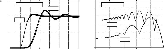
Step Response Overshoot
Butterworth and Chebyshev filters have an overshoot of 5 to 30% in their step responses, becoming larger as the number of poles is increased. Figure 20-3a shows the step response for two example Chebyshev filters. Figure (b) shows something that is unique to digital filters and has no counterpart in analog electronics: the amount of overshoot in the step response depends to a small degree on the cutoff frequency of the filter. The excessive overshoot and ringing in the step response results from the Chebyshev filter being optimized for the frequency domain at the expense of the time domain.
1.5 |
|
|
|
|
|
|
|
|
a. Step response |
|
|
|
|
||
|
|
|
|
4 pole |
|
|
|
1.0 |
|
|
|
|
|
|
|
Amplitude |
2 pole |
|
|
|
|
|
|
|
|
|
|
|
|
|
|
0.5 |
|
|
|
|
|
|
|
0.0 |
|
|
|
|
|
|
|
-10 |
0 |
10 |
20 |
30 |
40 |
50 |
60 |
Sample number
|
30 |
|
|
|
|
|
|
|
b. Overshoot |
|
|
|
|
overshoot |
25 |
|
|
|
|
|
20 |
|
|
|
|
|
|
|
|
|
|
|
|
|
Percent |
15 |
6 pole |
|
|
|
|
10 |
|
|
|
|
|
|
|
|
|
|
|
|
|
|
5 |
|
2 pole |
|
|
|
|
0 |
|
|
|
|
|
|
0 |
0.1 |
0.2 |
0.3 |
0.4 |
0.5 |
|
|
|
Frequency |
|
|
|
FIGURE 20-3
Chebyshev step response. The overshoot in the Chebyshev filter's step response is 5% to 30%, depending on the number of poles, as shown in (a), and the cutoff frequency, as shown in (b). Figure
(a) is for a cutoff frequency of 0.05, and may be scaled to other cutoff frequencies.
Chapter 20Chebyshev Filters |
339 |
Stability
The main limitation of digital filters carried out by convolution is execution time. It is possible to achieve nearly any filter response, provided you are willing to wait for the result. Recursive filters are just the opposite. They run like lightning; however, they are limited in performance. For example, consider a 6 pole, 0.5% ripple, low-pass filter with a 0.01 cutoff frequency. The recursion coefficients for this filter can be obtained from Table 20-1:
a0= 1.391351E-10
a1= 8.348109E-10 b1= 5.883343E+00 a2= 2.087027E-09 b2= -1.442798E+01 a3= 2.782703E-09 b3= 1.887786E+01 a4= 2.087027E-09 b4= -1.389914E+01 a5= 8.348109E-10 b5= 5.459909E+00 a6= 1.391351E-10 b6= -8.939932E-01
Look carefully at these coefficients. The "b" coefficients have an absolute value of about ten. Using single precision, the round-off noise on each of these numbers is about one ten-millionth of the value, i.e., 10&6 . Now look at the "a" coefficients, with a value of about 10&9 . Something is obviously wrong here. The contribution from the input signal (via the "a" coefficients) will be 1000 times smaller than the noise from the previously calculated output signal (via the "b" coefficients). This filter won't work! In short, round-off noise limits the number of poles that can be used in a filter. The actual number will depend slightly on the ripple and if it is a high or low-pass filter. The approximate numbers for single precision are:
TABLE 20-3 |
Cutoff frequency |
0.02 |
0.05 |
0.10 |
0.25 |
0.40 |
0.45 |
0.48 |
The maximum number of |
|
|
|
|
|
|
|
|
|
|
|
|
|
|
|
|
|
poles for single precision. |
Maximum poles |
4 |
6 |
10 |
20 |
10 |
6 |
4 |
|
The filter's performance will start to degrade as this limit is approached; the step response will show more overshoot, the stopband attenuation will be poor, and the frequency response will have excessive ripple. If the filter is pushed too far, or there is an error in the coefficients, the output will probably oscillate until an overflow occurs.
There are two ways of extending the maximum number of poles that can be used. First, use double precision. This requires using double precision in the coefficient calculation as well (including the value for pi ).
The second method is to implement the filter in stages. For example, a six pole filter starts out as a cascade of three stages of two poles each. The program in Table 20-4 combines these three stages into a single set of recursion coefficients for easier programming. However, the filter is more stable if carried out as the original three separate stages. This requires knowing the "a" and "b" coefficients for each of the stages. These can
340 |
The Scientist and Engineer's Guide to Digital Signal Processing |
||||
100 'CHEBYSHEV FILTERRECURSION COEFFICIENT CALCULATION |
|||||
110 |
' |
|
|
|
|
120 |
|
|
|
|
'INITIALIZE VARIABLES |
130 |
DIM A[22] |
|
|
|
'holds the "a" coefficients upon program completion |
140 |
DIM B[22] |
|
|
|
'holds the "b" coefficients upon program completion |
150 |
DIM TA[22] |
|
|
|
'internal use for combining stages |
160 |
DIM TB[22] |
|
|
|
'internal use for combining stages |
170 |
' |
|
|
|
|
180 FOR I% = 0 TO 22 |
|
|
|
||
190 |
A[I%] = 0 |
|
|
|
|
200 |
B[I%] = 0 |
|
|
|
|
210 NEXT I% |
|
|
|
|
|
220 |
' |
|
|
|
|
230 |
A[2] = 1 |
|
|
|
|
240 |
B[2] = 1 |
|
|
|
|
250 |
PI = 3.14159265 |
|
|
|
|
260 |
|
|
|
|
'ENTER THE FOUR FILTER PARAMETERS |
270 |
INPUT "Enter cutoff frequency |
(0 to .5): ", FC |
|||
280 |
INPUT "Enter |
0 for LP, 1 for HP filter: |
", LH |
||
290 |
INPUT "Enter percent ripple |
(0 to 29): |
", PR |
||
300 |
INPUT "Enter number of poles (2,4,...20): |
", NP |
|||
310 |
' |
|
|
|
|
320 FOR P% = 1 TO NP/2 |
|
|
'LOOP FOR EACH POLE-PAIR |
||
330 |
' |
|
|
|
|
340 |
GOSUB 1000 |
|
|
'The subroutine in TABLE 20-5 |
|
350 |
' |
|
|
|
|
360 |
FOR I% = 0 TO 22 |
|
|
'Add coefficients to the cascade |
|
370 |
TA[I%] = A[I%] |
|
|
|
|
380 |
TB[I%] = B[I%] |
|
|
|
|
390 |
NEXT I% |
|
|
|
|
400 |
' |
|
|
|
|
410 |
FOR I% = 2 TO 22 |
|
|
|
|
420 |
A[I%] = A0*TA[I%] + A1*TA[I%-1] + A2*TA[I%-2] |
||||
430 |
B[I%] = |
TB[I%] - B1*TB[I%-1] - B2*TB[I%-2] |
|||
440 |
NEXT I% |
|
|
|
|
450 |
' |
|
|
|
|
460 NEXT P% |
|
|
|
|
|
470 |
' |
|
|
|
|
480 |
B[2] = 0 |
|
|
|
'Finish combining coefficients |
490 FOR I% = 0 TO 20 |
|
|
|
||
500 |
A[I%] = A[I%+2] |
|
|
|
|
510 |
B[I%] = -B[I%+2] |
|
|
|
|
520 NEXT I% |
|
|
|
|
|
530 |
' |
|
|
|
|
540 SA = 0 |
|
|
|
'NORMALIZE THE GAIN |
|
550 |
SB = 0 |
|
|
|
|
560 FOR I% = 0 TO 20 |
|
|
|
||
570 |
IF LH = 0 THEN SA |
= SA |
+ A[I%] |
|
|
580 |
IF LH = 0 THEN SB |
= SB |
+ B[I%] |
|
|
590 |
IF LH = 1 THEN SA |
= SA |
+ A[I%] * (-1)^I% |
||
600 |
IF LH = 1 THEN SB |
= SB |
+ B[I%] * (-1)^I% |
||
610 NEXT I% |
|
|
|
|
|
620 |
' |
|
|
|
|
630 |
GAIN = SA / (1 - SB) |
|
|
|
|
640 |
' |
|
|
|
|
650 FOR I% = 0 TO 20 |
|
|
|
||
660 |
A[I%] = A[I%] / GAIN |
|
|
||
670 NEXT I% |
|
|
|
|
|
680 |
' |
|
|
|
'The final recursion coefficients are in A[ ] and B[ ] |
690 END |
|
|
|
|
|
TABLE 20-4
|
|
Chapter 20Chebyshev Filters |
341 |
|
1000 'THIS SUBROUTINE IS CALLED FROM TABLE 20-4, LINE 340 |
|
|||
1010 ' |
|
|
|
|
1020 |
' |
Variables entering subroutine: |
PI, FC, LH, PR, HP, P% |
|
1030 |
' |
Variables exiting subroutine: |
A0, A1, A2, B1, B2 |
|
1040 |
' |
Variables used internally: |
RP, IP, ES, VX, KX, T, W, M, D, K, |
|
1050 ' |
|
X0, X1, X2, Y1, Y2 |
|
|
1060 ' |
|
|
|
|
1070 ' |
|
'Calculate the pole location on the unit circle |
|
|
1080 |
RP = -COS(PI/(NP*2) + (P%-1) * PI/NP) |
|
||
1090 |
IP = SIN(PI/(NP*2) + (P%-1) * PI/NP) |
|
|
|
1100 ' |
|
|
|
|
1110 ' |
|
'Warp from a circle to an ellipse |
|
|
1120 IF PR = 0 THEN GOTO 1210 |
|
|
||
1130 |
ES = SQR( (100 / (100-PR))^2 -1 ) |
|
|
|
1140 |
VX = (1/NP) * LOG( (1/ES) + SQR( (1/ES^2) + 1) ) |
|
||
1150 |
KX = (1/NP) * LOG( (1/ES) + SQR( (1/ES^2) - 1) ) |
|
||
1160 |
KX = (EXP(KX) + EXP(-KX))/2 |
|
|
|
1170 |
RP = RP * ( (EXP(VX) - EXP(-VX) ) /2 ) / KX |
|
||
1180 |
IP = IP * ( (EXP(VX) + EXP(-VX) ) /2 ) / KX |
|
||
1190 ' |
|
|
|
|
1200 ' |
|
's-domain to z-domain conversion |
|
|
1210 |
T = 2 * TAN(1/2) |
|
|
|
1220 |
W = 2*PI*FC |
|
|
|
1230 |
M = RP^2 + IP^2 |
|
|
|
1240 |
D = 4 - 4*RP*T + M*T^2 |
|
|
|
1250 |
X0 = T^2/D |
|
|
|
1260 |
X1 = 2*T^2/D |
|
|
|
1270 |
X2 = T^2/D |
|
|
|
1280 |
Y1 = (8 - 2*M*T^2)/D |
|
|
|
1290 |
Y2 = (-4 - 4*RP*T - M*T^2)/D |
|
|
|
1300 ' |
|
|
|
|
1310 ' |
|
'LP TO LP, or LP TO HP transform |
|
|
1320 |
IF LH = 1 THEN K = -COS(W/2 + 1/2) / COS(W/2 - 1/2) |
|
||
1330 |
IF LH = 0 THEN K = SIN(1/2 - W/2) / SIN(1/2 + W/2) |
|
||
1340 |
D = 1 + Y1*K - Y2*K^2 |
|
|
|
1350 |
A0 = (X0 - X1*K + X2*K^2)/D |
|
|
|
1360 |
A1 = (-2*X0*K + X1 + X1*K^2 - 2*X2*K)/D |
|
||
1370 |
A2 = (X0*K^2 - X1*K + X2)/D |
|
|
|
1380 |
B1 = (2*K + Y1 + Y1*K^2 - 2*Y2*K)/D |
|
|
|
1390 |
B2 = (-(K^2) - Y1*K + Y2)/D |
|
|
|
1400 IF LH = 1 THEN A1 = -A1
1410 IF LH = 1 THEN B1 = -B1 1420 '
1430 RETURN
TABLE 20-5
TABLE 20-4 and 20-5
Program to calculate the "a" and "b" coefficients for Chebyshev recursive filters. In lines 270-300, four parameters are entered into the program. The cutoff frequency, FC, is expressed as a fraction of the sampling frequency, and therefore must be in the range: 0 to 0.5. The variable, LH, is set to a value of one for a high-pass filter, and zero for a low-pass filter. The value entered for PR must be in the range of 0 to 29, corresponding to 0 to 29% ripple in the filter's frequency response. The number of poles in the filter, entered in the variable NP, must be an even integer between 2 and 20. At the completion of the program, the "a" and "b" coefficients are stored in the arrays A[ ] and B[ ] (a0 = A[0], a1 = A[1], etc.). TABLE 20-5 is a subroutine called from line 340 of the main program. Six variables are passed to this subroutine, and five variables are returned. Table 20-6 (next page) contains two sets of data to help debug this subroutine. The functions: COS and SIN, use radians, not degrees. The function: LOG is the natural (base e) logarithm. Declaring all floating point variables (including the value of B) to be double precision will allow more poles to be used. Tables 20-1 and 20-2 were generated with this program and can be used to test for proper operation. Chapter 33 describes the mathematical operation of this program.
342 |
The Scientist and Engineer's Guide to Digital Signal Processing |
|||||
|
DATA SET 1 |
DATA SET 2 |
||||
|
Enter the subroutine with these values: |
|
|
|
||
|
FC |
= |
0.1 |
FC |
= |
0.1 |
|
LH |
= |
0 |
LH |
= |
1 |
|
PR |
= |
0 |
PR |
= |
10 |
|
NP |
= |
4 |
NP |
= |
4 |
|
P% |
= |
1 |
P% |
= |
2 |
|
PI |
= |
3.141592 |
PI |
= |
3.141592 |
These values should be present at line 1200:
RP |
= -0.923879 |
RP |
= -0.136178 |
||
IP |
= |
0.382683 |
IP |
= |
0.933223 |
ES |
= |
not used |
ES |
= |
0.484322 |
VX |
= |
not used |
VX |
= |
0.368054 |
KX |
= |
not used |
KX |
= |
1.057802 |
These values should be present at line 1310:
T |
= |
1.092605 |
T |
= |
1.092605 |
W |
= |
0.628318 |
W |
= |
0.628318 |
M |
= |
1.000000 |
M |
= |
0.889450 |
D |
= |
9.231528 |
D |
= |
5.656972 |
X0 |
= |
0.129316 |
X0 |
= |
0.211029 |
X1 |
= |
0.258632 |
X1 |
= |
0.422058 |
X2 |
= |
0.129316 |
X2 |
= |
0.211029 |
Y1 |
= |
0.607963 |
Y1 |
= |
1.038784 |
Y2 |
= -0.125227 |
Y2 |
= -0.789584 |
||
These values should be return to the main program:
A0 |
= |
0.061885 |
A0 |
= |
0.922919 |
A1 |
= |
0.123770 |
A1 |
= -1.845840 |
|
A2 |
= |
0.061885 |
A2 |
= |
0.922919 |
B1 |
= |
1.048600 |
B1 |
= |
1.446913 |
B2 |
= |
-0.296140 |
B2 |
= |
-0.836653 |
TABLE 20-6
Debugging data. This table contains two sets of data for debugging the subroutine listed in Table 20-5.
be obtained from the program in Table 20-4. The subroutine in Table 20-5 is called once for each stage in the cascade. For example, it is called three times for a six pole filter. At the completion of the subroutine, five variables are return to the main program: A0, A1, A2, B1, & B2. These are the recursion coefficients for the two pole stage being worked on, and can be used to implement the filter in stages.