

CHAPTER
Statistics, Probability and Noise
2
Statistics and probability are used in Digital Signal Processing to characterize signals and the processes that generate them. For example, a primary use of DSP is to reduce interference, noise, and other undesirable components in acquired data. These may be an inherent part of the signal being measured, arise from imperfections in the data acquisition system, or be introduced as an unavoidable byproduct of some DSP operation. Statistics and probability allow these disruptive features to be measured and classified, the first step in developing strategies to remove the offending components. This chapter introduces the most important concepts in statistics and probability, with emphasis on how they apply to acquired signals.
Signal and Graph Terminology
A signal is a description of how one parameter is related to another parameter. For example, the most common type of signal in analog electronics is a voltage that varies with time. Since both parameters can assume a continuous range of values, we will call this a continuous signal. In comparison, passing this signal through an analog-to-digital converter forces each of the two parameters to be quantized. For instance, imagine the conversion being done with 12 bits at a sampling rate of 1000 samples per second. The voltage is curtailed to 4096 (212) possible binary levels, and the time is only defined at one millisecond increments. Signals formed from parameters that are quantized in this manner are said to be discrete signals or digitized signals. For the most part, continuous signals exist in nature, while discrete signals exist inside computers (although you can find exceptions to both cases). It is also possible to have signals where one parameter is continuous and the other is discrete. Since these mixed signals are quite uncommon, they do not have special names given to them, and the nature of the two parameters must be explicitly stated.
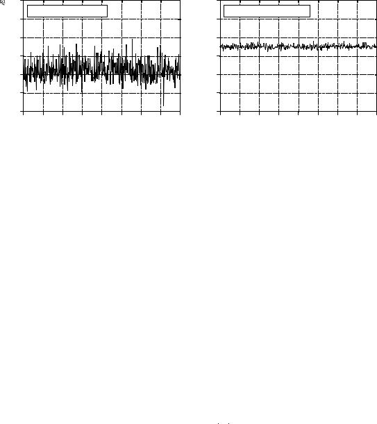
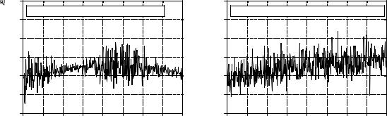
Figure 2-1 shows two discrete signals, such as might be acquired with a digital data acquisition system. The vertical axis may represent voltage, light
11
12 |
The Scientist and Engineer's Guide to Digital Signal Processing |
intensity, sound pressure, or an infinite number of other parameters. Since we don't know what it represents in this particular case, we will give it the generic label: amplitude. This parameter is also called several other names: the y- axis, the dependent variable, the range, and the ordinate.
The horizontal axis represents the other parameter of the signal, going by such names as: the x-axis, the independent variable, the domain, and the abscissa. Time is the most common parameter to appear on the horizontal axis of acquired signals; however, other parameters are used in specific applications. For example, a geophysicist might acquire measurements of rock density at equally spaced distances along the surface of the earth. To keep things general, we will simply label the horizontal axis: sample number. If this were a continuous signal, another label would have to be used, such as: time, distance, x, etc.
The two parameters that form a signal are generally not interchangeable. The parameter on the y-axis (the dependent variable) is said to be a function of the parameter on the x-axis (the independent variable). In other words, the independent variable describes how or when each sample is taken, while the dependent variable is the actual measurement. Given a specific value on the x-axis, we can always find the corresponding value on the y-axis, but usually not the other way around.
Pay particular attention to the word: domain, a very widely used term in DSP. For instance, a signal that uses time as the independent variable (i.e., the parameter on the horizontal axis), is said to be in the time domain. Another common signal in DSP uses frequency as the independent variable, resulting in the term, frequency domain. Likewise, signals that use distance as the independent parameter are said to be in the spatial domain (distance is a measure of space). The type of parameter on the horizontal axis is the domain of the signal; it's that simple. What if the x-axis is labeled with something very generic, such as sample number? Authors commonly refer to these signals as being in the time domain. This is because sampling at equal intervals of time is the most common way of obtaining signals, and they don't have anything more specific to call it.
Although the signals in Fig. 2-1 are discrete, they are displayed in this figure as continuous lines. This is because there are too many samples to be distinguishable if they were displayed as individual markers. In graphs that portray shorter signals, say less than 100 samples, the individual markers are usually shown. Continuous lines may or may not be drawn to connect the markers, depending on how the author wants you to view the data. For instance, a continuous line could imply what is happening between samples, or simply be an aid to help the reader's eye follow a trend in noisy data. The point is, examine the labeling of the horizontal axis to find if you are working with a discrete or continuous signal. Don't rely on an illustrator's ability to draw dots.
The variable, N, is widely used in DSP to represent the total number of samples in a signal. For example, N ' 512 for the signals in Fig. 2-1. To
Chapter 2- Statistics, Probability and Noise |
13 |
|
8 |
|
|
|
|
|
|
|
|
|
6 |
a. Mean = 0.5, F = 1 |
|
|
|
|
|
||
|
|
|
|
|
|
|
|
|
|
Amplitude |
4 |
|
|
|
|
|
|
|
|
2 |
|
|
|
|
|
|
|
|
|
|
|
|
|
|
|
|
|
|
|
|
0 |
|
|
|
|
|
|
|
|
|
-2 |
|
|
|
|
|
|
|
|
|
-4 |
|
|
|
|
|
|
|
|
|
0 |
64 |
128 |
192 |
256 |
320 |
384 |
448 |
5121 |
Sample number
|
8 |
|
|
|
|
|
|
|
|
|
|
b. Mean = 3.0, F = 0.2 |
|
|
|
|
|||
|
6 |
|
|
|
|
|
|
|
|
Amplitude |
4 |
|
|
|
|
|
|
|
|
2 |
|
|
|
|
|
|
|
|
|
0 |
|
|
|
|
|
|
|
|
|
|
|
|
|
|
|
|
|
|
|
|
-2 |
|
|
|
|
|
|
|
|
|
-4 |
|
|
|
|
|
|
|
|
|
0 |
64 |
128 |
192 |
256 |
320 |
384 |
448 |
5121 |
Sample number
FIGURE 2-1
Examples of two digitized signals with different means and standard deviations.
keep the data organized, each sample is assigned a sample number or index. These are the numbers that appear along the horizontal axis. Two notations for assigning sample numbers are commonly used. In the first notation, the sample indexes run from 1 to N (e.g., 1 to 512). In the second notation, the sample indexes run from 0 to N & 1 (e . g . , 0 to 511) . Mathematicians often use the first method (1 to N), while those in DSP commonly uses the second (0 to N & 1 ). In this book, we will use the second notation. Don't dismiss this as a trivial problem. It will confuse you sometime during your career. Look out for it!
Mean and Standard Deviation
The mean, indicated by µ (a lower case Greek mu), is the statistician's jargon for the average value of a signal. It is found just as you would expect: add all of the samples together, and divide by N. It looks like this in mathematical form:
EQUATION 2-1
Calculation of a signal's mean. The signal is contained in x0 through xN-1, i is an index that runs through these values, and µ is the mean.
|
1 |
N & 1 |
|
µ ' |
j xi |
||
|
|||
N |
|||
|
i ' 0 |
In words, sum the values in the signal, xi , by letting the index, i, run from 0 to N & 1 . Then finish the calculation by dividing the sum by N. This is identical to the equation: µ ' (x0% x1% x2% þ% xN & 1) /N . If you are not already familiar with E (upper case Greek sigma) being used to indicate summation, study these equations carefully, and compare them with the computer program in Table 2-1. Summations of this type are abundant in DSP, and you need to understand this notation fully.
14 |
The Scientist and Engineer's Guide to Digital Signal Processing |
In electronics, the mean is commonly called the DC (direct current) value. Likewise, AC (alternating current) refers to how the signal fluctuates around the mean value. If the signal is a simple repetitive waveform, such as a sine or square wave, its excursions can be described by its peak-to-peak amplitude. Unfortunately, most acquired signals do not show a well defined peak-to-peak value, but have a random nature, such as the signals in Fig. 2-1. A more generalized method must be used in these cases, called the standard deviation, denoted by F (a lower case Greek sigma).
As a starting point, the expression,*xi & µ *, describes how far the i th sample deviates (differs) from the mean. The average deviation of a signal is found by summing the deviations of all the individual samples, and then dividing by the number of samples, N. Notice that we take the absolute value of each deviation before the summation; otherwise the positive and negative terms would average to zero. The average deviation provides a single number representing the typical distance that the samples are from the mean. While convenient and straightforward, the average deviation is almost never used in statistics. This is because it doesn't fit well with the physics of how signals operate. In most cases, the important parameter is not the deviation from the mean, but the power represented by the deviation from the mean. For example, when random noise signals combine in an electronic circuit, the resultant noise is equal to the combined power of the individual signals, not their combined amplitude.
The standard deviation is similar to the average deviation, except the averaging is done with power instead of amplitude. This is achieved by squaring each of the deviations before taking the average (remember, power % voltage2). To finish, the square root is taken to compensate for the initial squaring. In equation form, the standard deviation is calculated:
EQUATION 2-2 |
|
|
|
|
N & 1 |
|
|
|
|
|
Calculation of the standard deviation of a |
|
|
|
|
|
|
|
|
|
|
F2 ' |
|
1 |
|
j(xi |
& µ )2 |
|
|
|
|
|
signal. The signal is stored in xi , µ is the |
|
|
|
|
|
|
||||
N & 1 |
|
|
|
|
||||||
mean found from Eq. 2-1, N is the number of |
|
i ' 0 |
|
|
|
|
|
|||
samples, and σ is the standard deviation. |
|
|
|
|
|
|
|
|
|
|
|
notation: F' |
|
|
|
|
|
|
|||
In the alternative |
|
(x & µ )2 % (x & µ )2 % þ% (x |
N & 1 |
& µ )2 |
/ (N & 1). |
|||||
|
|
|
|
|
0 |
1 |
|
|
|
|
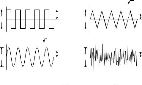
Notice that the average is carried out by dividing by N & 1 instead of N. This is a subtle feature of the equation that will be discussed in the next section. The term, F2, occurs frequently in statistics and is given the name variance. The standard deviation is a measure of how far the signal fluctuates from the mean. The variance represents the power of this fluctuation. Another term you should become familiar with is the rms (root-mean-square) value, frequently used in electronics. By definition, the standard deviation only measures the AC portion of a signal, while the rms value measures both the AC and DC components. If a signal has no DC component, its rms value is identical to its standard deviation. Figure 2-2 shows the relationship between the standard deviation and the peak-to-peak value of several common waveforms.
Chapter 2- Statistics, Probability and Noise |
15 |
a. Square Wave, Vpp = 2F |
b. Triangle wave, Vpp = |
12 F |
|
|
|
F |
F |
Vpp |
|
Vpp |
|
|
|
||
c. Sine wave, Vpp = 2 |
2 F |
d. Random noise, Vpp . 6-8 F |
|
F |
F |
Vpp |
Vpp |
FIGURE 2-2
Ratio of the peak-to-peak amplitude to the standard deviation for several common waveforms. For the square wave, this ratio is 2; for the triangle wave it is  12 ' 3.46 ; for the sine wave it is 2
 2 ' 2.83 . While random noise has no exact peak-to-peak value, it is approximately 6 to 8 times the standard deviation.
Table 2-1 lists a computer routine for calculating the mean and standard deviation using Eqs. 2-1 and 2-2. The programs in this book are intended to convey algorithms in the most straightforward way; all other factors are treated as secondary. Good programming techniques are disregarded if it makes the program logic more clear. For instance: a simplified version of BASIC is used, line numbers are included, the only control structure allowed is the FOR-NEXT loop, there are no I/O statements, etc. Think of these programs as an alternative way of understanding the equations used
100 CALCULATION OF THE MEAN AND STANDARD DEVIATION
110 |
' |
|
120 |
DIM X[511] |
'The signal is held in X[0] to X[511] |
130 N% = 512 |
'N% is the number of points in the signal |
|
140 |
' |
|
150 |
GOSUB XXXX |
'Mythical subroutine that loads the signal into X[ ] |
160 |
' |
|
170 |
MEAN = 0 |
'Find the mean via Eq. 2-1 |
180 FOR I% = 0 TO N%-1 |
|
|
190 |
MEAN = MEAN + X[I%] |
|
200 NEXT I% |
|
|
210 MEAN = MEAN/N% |
|
|
220 |
' |
|
230 |
VARIANCE = 0 |
'Find the standard deviation via Eq. 2-2 |
240 FOR I% = 0 TO N%-1 |
|
|
250 |
VARIANCE = VARIANCE + ( X[I%] - MEAN )^2 |
|
260 NEXT I%
270 VARIANCE = VARIANCE/(N%-1)
280 SD = SQR(VARIANCE) |
|
290 ' |
|
300 PRINT MEAN SD |
'Print the calculated mean and standard deviation |
310 ' |
|
320 END
TABLE 2-1
16 |
The Scientist and Engineer's Guide to Digital Signal Processing |
in DSP. If you can't grasp one, maybe the other will help. In BASIC, the % character at the end of a variable name indicates it is an integer. All other variables are floating point. Chapter 4 discusses these variable types in detail.
This method of calculating the mean and standard deviation is adequate for many applications; however, it has two limitations. First, if the mean is much larger than the standard deviation, Eq. 2-2 involves subtracting two numbers that are very close in value. This can result in excessive round-off error in the calculations, a topic discussed in more detail in Chapter 4. Second, it is often desirable to recalculate the mean and standard deviation as new samples are acquired and added to the signal. We will call this type of calculation: running statistics. While the method of Eqs. 2-1 and 2-2 can be used for running statistics, it requires that all of the samples be involved in each new calculation. This is a very inefficient use of computational power and memory.
A solution to these problems can be found by manipulating Eqs. 2-1 and 2-2 to provide another equation for calculating the standard deviation:
EQUATION 2-3
Calculation of the standard deviation using running statistics. This equation provides the same result as Eq. 2-2, but with less round- o f f n o i s e a n d g r e a t e r c o m p u t a t i o n a l efficiency. The signal is expressed in terms of three accumulated parameters: N, the total number of samples; sum, the sum of these samples; and sum of squares, the sum of the squares of the samples. The mean and standard deviation are then calculated from these three accumulated parameters.
|
|
|
|
|
|
|
N &1 |
|
|
N &1 |
2 |
|
F2 ' |
1 |
|
|
|
j xi2 & |
1 |
|
j xi |
|
|||
|
|
|
||||||||||
N & 1 |
N |
|
|
|||||||||
|
|
|
||||||||||
|
|
|
|
i' 0 |
|
i '0 |
|
|||||
|
|
|
or using a simpler notation, |
|
|
|
||||||
F2 |
' |
1 |
|
|
sum of squares |
& |
|
sum 2 |
|
|||
|
|
|
|
|||||||||
|
|
|
||||||||||
N & 1 |
|
|
N |
|
||||||||
|
|
|
||||||||||
|
|
|
|
|
|
|
|
|
||||
While moving through the signal, a running tally is kept of three parameters:
(1) the number of samples already processed, (2) the sum of these samples, and (3) the sum of the squares of the samples (that is, square the value of each sample and add the result to the accumulated value). After any number of samples have been processed, the mean and standard deviation can be efficiently calculated using only the current value of the three parameters. Table 2-2 shows a program that reports the mean and standard deviation in this manner as each new sample is taken into account. This is the method used in hand calculators to find the statistics of a sequence of numbers. Every time you enter a number and press the E (summation) key, the three parameters are updated. The mean and standard deviation can then be found whenever desired, without having to recalculate the entire sequence.
|
Chapter 2- Statistics, Probability and Noise |
17 |
|
100 'MEAN AND STANDARD DEVIATION USING RUNNING STATISTICS |
|
||
110 ' |
|
|
|
120 |
DIM X[511] |
'The signal is held in X[0] to X[511] |
|
130 ' |
|
|
|
140 |
GOSUB XXXX |
'Mythical subroutine that loads the signal into X[ ] |
|
150 ' |
|
|
|
160 N% = 0 |
'Zero the three running parameters |
|
|
170 SUM = 0 |
|
|
|
180 SUMSQUARES = 0 |
|
|
|
190 ' |
|
|
|
200 |
FOR I% = 0 TO 511 |
'Loop through each sample in the signal |
|
210 |
' |
|
|
220 |
N% = N%+1 |
'Update the three parameters |
|
230 |
SUM = SUM + X[I%] |
|
|
240 |
SUMSQUARES = SUMSQUARES + X[I%]^2 |
|
|
250 |
' |
|
|
260 |
MEAN = SUM/N% |
'Calculate mean and standard deviation via Eq. 2-3 |
|
270 |
IF N% = 1 THEN SD = 0: GOTO 300 |
|
|
280 |
SD = SQR( (SUMSQUARES - SUM^2/N%) / (N%-1) ) |
|
|
290 |
' |
|
|
300 |
PRINT MEAN SD |
'Print the running mean and standard deviation |
|
310 |
' |
|
|
320 NEXT I%
330 '
340 END
TABLE 2-2
Before ending this discussion on the mean and standard deviation, two other terms need to be mentioned. In some situations, the mean describes what is being measured, while the standard deviation represents noise and other interference. In these cases, the standard deviation is not important in itself, but only in comparison to the mean. This gives rise to the term: signal-to-noise ratio (SNR), which is equal to the mean divided by the standard deviation. Another term is also used, the coefficient of variation (CV). This is defined as the standard deviation divided by the mean, multiplied by 100 percent. For example, a signal (or other group of measure values) with a CV of 2%, has an SNR of 50. Better data means a higher value for the SNR and a lower value for the CV.
Signal vs. Underlying Process
Statistics is the science of interpreting numerical data, such as acquired signals. In comparison, probability is used in DSP to understand the processes that generate signals. Although they are closely related, the distinction between the acquired signal and the underlying process is key to many DSP techniques.
For example, imagine creating a 1000 point signal by flipping a coin 1000 times. If the coin flip is heads, the corresponding sample is made a value of one. On tails, the sample is set to zero. The process that created this signal has a mean of exactly 0.5, determined by the relative probability of each possible outcome: 50% heads, 50% tails. However, it is unlikely that the actual 1000 point signal will have a mean of exactly 0.5. Random chance

18 |
The Scientist and Engineer's Guide to Digital Signal Processing |
will make the number of ones and zeros slightly different each time the signal is generated. The probabilities of the underlying process are constant, but the statistics of the acquired signal change each time the experiment is repeated. This random irregularity found in actual data is called by such names as: statistical variation, statistical fluctuation, and statistical noise.
This presents a bit of a dilemma. When you see the terms: mean and standard deviation, how do you know if the author is referring to the statistics of an actual signal, or the probabilities of the underlying process that created the signal? Unfortunately, the only way you can tell is by the context. This is not so for all terms used in statistics and probability. For example, the histogram and probability mass function (discussed in the next section) are matching concepts that are given separate names.
Now, back to Eq. 2-2, calculation of the standard deviation. As previously mentioned, this equation divides by N-1 in calculating the average of the squared deviations, rather than simply by N. To understand why this is so, imagine that you want to find the mean and standard deviation of some process that generates signals. Toward this end, you acquire a signal of N samples from the process, and calculate the mean of the signal via Eq. 2.1. You can then use this as an estimate of the mean of the underlying process; however, you know there will be an error due to statistical noise. In particular, for random signals, the typical error between the mean of the N points, and the mean of the underlying process, is given by:
EQUATION 2-4
Typical error in calculating the mean of an underlying process by using a finite number of samples, N. The parameter, σ , is the standard deviation.
F
Typical error '
N 1/2
If N is small, the statistical noise in the calculated mean will be very large. In other words, you do not have access to enough data to properly characterize the process. The larger the value of N, the smaller the expected error will become. A milestone in probability theory, the Strong Law of Large Numbers, guarantees that the error becomes zero as N approaches infinity.
In the next step, we would like to calculate the standard deviation of the acquired signal, and use it as an estimate of the standard deviation of the underlying process. Herein lies the problem. Before you can calculate the standard deviation using Eq. 2-2, you need to already know the mean, µ. However, you don't know the mean of the underlying process, only the mean of the N point signal, which contains an error due to statistical noise. This error tends to reduce the calculated value of the standard deviation. To compensate for this, N is replaced by N-1. If N is large, the difference doesn't matter. If N is small, this replacement provides a more accurate
Chapter 2- Statistics, Probability and Noise |
19 |
|
8 |
|
|
|
|
|
|
|
|
|
|
a. Changing mean and standard deviation |
|
|
|||||
|
6 |
|
|
|
|
|
|
|
|
Amplitude |
4 |
|
|
|
|
|
|
|
|
2 |
|
|
|
|
|
|
|
|
|
0 |
|
|
|
|
|
|
|
|
|
|
|
|
|
|
|
|
|
|
|
|
-2 |
|
|
|
|
|
|
|
|
|
-4 |
|
|
|
|
|
|
|
|
|
0 |
64 |
128 |
192 |
256 |
320 |
384 |
448 |
5121 |
Sample number
|
8 |
|
|
|
|
|
|
|
|
|
|
b. Changing mean, constant standard deviation |
|
||||||
|
6 |
|
|
|
|
|
|
|
|
Amplitude |
4 |
|
|
|
|
|
|
|
|
2 |
|
|
|
|
|
|
|
|
|
0 |
|
|
|
|
|
|
|
|
|
|
|
|
|
|
|
|
|
|
|
|
-2 |
|
|
|
|
|
|
|
|
|
-4 |
|
|
|
|
|
|
|
|
|
0 |
64 |
128 |
192 |
256 |
320 |
384 |
448 |
5121 |
Sample number
FIGURE 2-3
Examples of signals generated from nonstationary processes. In (a), both the mean and standard deviation change. In (b), the standard deviation remains a constant value of one, while the mean changes from a value of zero to two. It is a common analysis technique to break these signals into short segments, and calculate the statistics of each segment individually.
estimate of the standard deviation of the underlying process. In other words, Eq. 2-2 is an estimate of the standard deviation of the underlying process. If we divided by N in the equation, it would provide the standard deviation of the acquired signal.
As an illustration of these ideas, look at the signals in Fig. 2-3, and ask: are the variations in these signals a result of statistical noise, or is the underlying process changing? It probably isn't hard to convince yourself that these changes are too large for random chance, and must be related to the underlying process. Processes that change their characteristics in this manner are called nonstationary. In comparison, the signals previously presented in Fig. 2-1 were generated from a stationary process, and the variations result completely from statistical noise. Figure 2-3b illustrates a common problem with nonstationary signals: the slowly changing mean interferes with the calculation of the standard deviation. In this example, the standard deviation of the signal, over a short interval, is one. However, the standard deviation of the entire signal is 1.16. This error can be nearly eliminated by breaking the signal into short sections, and calculating the statistics for each section individually. If needed, the standard deviations for each of the sections can be averaged to produce a single value.
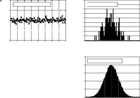
The Histogram, Pmf and Pdf
Suppose we attach an 8 bit analog-to-digital converter to a computer, and acquire 256,000 samples of some signal. As an example, Fig. 2-4a shows 128 samples that might be a part of this data set. The value of each sample will be one of 256 possibilities, 0 through 255. The histogram displays the number of samples there are in the signal that have each of these possible values. Figure (b) shows the histogram for the 128 samples in (a). For
20 |
The Scientist and Engineer's Guide to Digital Signal Processing |
|
255 |
|
|
a. 128 samples of 8 bit signal |
|
Amplitude |
192 |
|
128 |
||
|
64 


0
0 |
16 |
32 |
48 |
64 |
80 |
96 |
112 |
1287 |
Sample number
 Number of occurences
9
8  b. 128 point histogram
7
6
5
4
3
2
1
0
90 |
100 |
110 |
120 |
130 |
140 |
150 |
160 |
170 |
Value of sample
FIGURE 2-4
Examples of histograms. Figure (a) shows 128 samples from a very long signal, with each sample being an integer between 0 and 255. Figures (b) and (c) show histograms using 128 and 256,000 samples from the signal, respectively. As shown, the histogram is smoother when more samples are used.
10000
|
c. 256,000 point histogram |
|
occurencesof |
8000 |
|
6000 |
||
Number |
||
4000 |
||
|
||
|
2000 |
0 |
|
|
|
|
|
|
|
|
90 |
100 |
110 |
120 |
130 |
140 |
150 |
160 |
170 |
Value of sample
example, there are 2 samples that have a value of 110, 7 samples that have a value of 131, 0 samples that have a value of 170, etc. We will represent the histogram by Hi, where i is an index that runs from 0 to M-1, and M is the number of possible values that each sample can take on. For instance, H50 is the number of samples that have a value of 50. Figure (c) shows the histogram of the signal using the full data set, all 256k points. As can be seen, the larger number of samples results in a much smoother appearance. Just as with the mean, the statistical noise (roughness) of the histogram is inversely proportional to the square root of the number of samples used.
From the way it is defined, the sum of all of the values in the histogram must be equal to the number of points in the signal:
EQUATION 2-5
The sum of all of the values in the histogram is equal to the number of points in the signal. In this equation, Hi is the histogram, N is the number of points in the signal, and M is the number of points in the histogram.
M&1
N ' j Hi
i ' 0
The histogram can be used to efficiently calculate the mean and standard deviation of very large data sets. This is especially important for images, which can contain millions of samples. The histogram groups samples