

Chapter 2- Statistics, Probability and Noise |
21 |
together that have the same value. This allows the statistics to be calculated by working with a few groups, rather than a large number of individual samples. Using this approach, the mean and standard deviation are calculated from the histogram by the equations:
EQUATION 2-6
Calculation of the mean from the histogram. This can be viewed as combining all samples having the same value into groups, and then using Eq. 2-1 on each group.
EQUATION 2-7
Calculation of the standard deviation from the histogram. This is the same concept as Eq. 2-2, except that all samples having the same value are operated on at once.
|
|
1 |
M&1 |
||
µ |
' |
j i Hi |
|||
|
|
||||
N |
|||||
|
|
i ' 0 |
|||
|
1 |
|
M &1 |
||
F2 ' |
|
j (i & µ )2 Hi |
|||
|
|
||||
|
|
||||
|
N & 1 i '0 |
||||
Table 2-3 contains a program for calculating the histogram, mean, and standard deviation using these equations. Calculation of the histogram is very fast, since it only requires indexing and incrementing. In comparison,
100 |
'CALCULATION OF THE HISTOGRAM, MEAN, AND STANDARD DEVIATION |
|
110 |
' |
|
120 |
DIM X%[25000] |
'X%[0] to X%[25000] holds the signal being processed |
130 |
DIM H%[255] |
'H%[0] to H%[255] holds the histogram |
140 N% = 25001 |
'Set the number of points in the signal |
|
150 |
' |
|
160 |
FOR I% = 0 TO 255 |
'Zero the histogram, so it can be used as an accumulator |
170 |
H%[I%] = 0 |
|
180 NEXT I% |
|
|
190 |
' |
|
200 |
GOSUB XXXX |
'Mythical subroutine that loads the signal into X%[ ] |
210 |
' |
|
220 |
FOR I% = 0 TO 25000 'Calculate the histogram for 25001 points |
|
230 |
H%[ X%[I%] ] = H%[ X%[I%] ] + 1 |
|
240 NEXT I% |
|
|
250 |
' |
|
260 |
MEAN = 0 |
'Calculate the mean via Eq. 2-6 |
270 FOR I% = 0 TO 255 |
|
|
280 |
MEAN = MEAN + I% * H%[I%] |
|
290 NEXT I% |
|
|
300 MEAN = MEAN / N% |
|
|
310 |
' |
|
320 |
VARIANCE = 0 |
'Calculate the standard deviation via Eq. 2-7 |
330 FOR I% = 0 TO 255 |
|
|
340 |
VARIANCE = VARIANCE + H%[I%] * (I%-MEAN)^2 |
|
350 NEXT I% |
|
|
360 VARIANCE = VARIANCE / (N%-1) |
||
370 SD = SQR(VARIANCE) |
|
|
380 |
' |
|
390 |
PRINT MEAN SD |
'Print the calculated mean and standard deviation. |
400 |
' |
|
410 END |
TABLE 2-3 |
|
|
|
|
22 |
The Scientist and Engineer's Guide to Digital Signal Processing |
calculating the mean and standard deviation requires the time consuming operations of addition and multiplication. The strategy of this algorithm is to use these slow operations only on the few numbers in the histogram, not the many samples in the signal. This makes the algorithm much faster than the previously described methods. Think a factor of ten for very long signals with the calculations being performed on a general purpose computer.
The notion that the acquired signal is a noisy version of the underlying process is very important; so important that some of the concepts are given different names. The histogram is what is formed from an acquired signal. The corresponding curve for the underlying process is called the probability mass function (pmf). A histogram is always calculated using a finite number of samples, while the pmf is what would be obtained with an infinite number of samples. The pmf can be estimated (inferred) from the histogram, or it may be deduced by some mathematical technique, such as in the coin flipping example.
Figure 2-5 shows an example pmf, and one of the possible histograms that could be associated with it. The key to understanding these concepts rests in the units of the vertical axis. As previously described, the vertical axis of the histogram is the number of times that a particular value occurs in the signal. The vertical axis of the pmf contains similar information, except expressed on a fractional basis. In other words, each value in the histogram is divided by the total number of samples to approximate the pmf. This means that each value in the pmf must be between zero and one, and that the sum of all of the values in the pmf will be equal to one.
The pmf is important because it describes the probability that a certain value will be generated. For example, imagine a signal with the pmf of Fig. 2-5b, such as previously shown in Fig. 2-4a. What is the probability that a sample taken from this signal will have a value of 120? Figure 2-5b provides the answer, 0.03, or about 1 chance in 34. What is the probability that a randomly chosen sample will have a value greater than 150? Adding up the values in the pmf for: 151, 152, 153,@@@, 255, provides the answer, 0.0122, or about 1 chance in 82. Thus, the signal would be expected to have a value exceeding 150 on an average of every 82 points. What is the probability that any one sample will be between 0 and 255? Summing all of the values in the pmf produces the probability of 1.00, that is, a certainty that this will occur.
The histogram and pmf can only be used with discrete data, such as a digitized signal residing in a computer. A similar concept applies to continuous signals, such as voltages appearing in analog electronics. The probability density function (pdf), also called the probability distribution function, is to continuous signals what the probability mass function is to discrete signals. For example, imagine an analog signal passing through an analog-to-digital converter, resulting in the digitized signal of Fig. 2-4a. For simplicity, we will assume that voltages between 0 and 255 millivolts become digitized into digital numbers between 0 and 255. The pmf of this digital

Chapter 2- Statistics, Probability and Noise |
23 |
|
10000 |
|
|
|
|
|
|
|
|
|
0.060 |
|
|
|
|
|
|
|
|
|
|
a. Histogram |
|
|
|
|
|
|
|
|
b. Probability Mass Function (pmf) |
|
|
||||||
Number of occurences |
8000 |
|
|
|
|
|
|
|
|
Probability of occurence |
0.050 |
|
|
|
|
|
|
|
|
|
|
|
|
|
|
|
|
|
|
|
|
|
|
|
|
|
|||
|
|
|
|
|
|
|
|
|
0.040 |
|
|
|
|
|
|
|
|
||
6000 |
|
|
|
|
|
|
|
|
|
|
|
|
|
|
|
|
|
||
|
|
|
|
|
|
|
|
|
0.030 |
|
|
|
|
|
|
|
|
||
4000 |
|
|
|
|
|
|
|
|
|
|
|
|
|
|
|
|
|
||
|
|
|
|
|
|
|
|
|
0.020 |
|
|
|
|
|
|
|
|
||
2000 |
|
|
|
|
|
|
|
|
0.010 |
|
|
|
|
|
|
|
|
||
|
|
|
|
|
|
|
|
|
|
|
|
|
|
|
|
|
|
||
|
|
|
|
|
|
|
|
|
|
|
|
|
|
|
|
|
|
|
|
|
0 |
|
|
|
|
|
|
|
|
|
0.000 |
|
|
|
|
|
|
|
|
|
90 |
100 |
110 |
120 |
130 |
140 |
150 |
160 |
170 |
|
90 |
100 |
110 |
120 |
130 |
140 |
150 |
160 |
170 |
Value of sample |
Value of sample |
FIGURE 2-5
The relationship between (a) the histogram, (b) the probability mass function (pmf), and (c) the probability density function (pdf). The histogram is calculated from a finite number of samples. The pmf describes the probabilities of the underlying process. The pdf is similar to the pmf, but is used with continuous rather than discrete signals. Even though the vertical axis of (b) and (c) have the same values (0 to 0.06), this is only a coincidence of this example. The amplitude of these three curves is determined by:
(a) the sum of the values in the histogram being equal to the number of samples in the signal; (b) the sum of the values in the pmf being equal to one, and (c) the area under the pdf curve being equal to one.
 Probability density
0.060
c. Probability Density Function (pdf)
0.050
0.040
0.030
0.020
0.010
0.000
90 |
100 |
110 |
120 |
130 |
140 |
150 |
160 |
170 |
Signal level (millivolts)
signal is shown by the markers in Fig. 2-5b. Similarly, the pdf of the analog signal is shown by the continuous line in (c), indicating the signal can take on a continuous range of values, such as the voltage in an electronic circuit.
The vertical axis of the pdf is in units of probability density, rather than just probability. For example, a pdf of 0.03 at 120.5 does not mean that the a voltage of 120.5 millivolts will occur 3% of the time. In fact, the probability of the continuous signal being exactly 120.5 millivolts is infinitesimally small. This is because there are an infinite number of possible values that the signal needs to divide its time between: 120.49997, 120.49998, 120.49999, etc. The chance that the signal happens to be exactly 120.50000þ is very remote indeed!
To calculate a probability, the probability density is multiplied by a range of values. For example, the probability that the signal, at any given instant, will be between the values of 120 and 121 is: (121&120) × 0.03 ' 0.03. The p r o b a b i l i t y t h a t t h e s i g n a l w i l l b e b e t w e e n 1 2 0 . 4 a n d 1 2 0 . 5 i s : (120.5&120.4) × 0.03 ' 0.003 , etc. If the pdf is not constant over the range of interest, the multiplication becomes the integral of the pdf over that range. In other words, the area under the pdf bounded by the specified values. Since the value of the signal must always be something, the total area under the pdf

24 |
The Scientist and Engineer's Guide to Digital Signal Processing |
curve, the integral from &4 to %4, will always be equal to one. This is analogous to the sum of all of the pmf values being equal to one, and the sum of all of the histogram values being equal to N.
The histogram, pmf, and pdf are very similar concepts. Mathematicians always keep them straight, but you will frequently find them used interchangeably (and therefore, incorrectly) by many scientists and
FIGURE 2-6
Three common waveforms and their probability density functions. As in these examples, the pdf graph is often rotated one-quarter turn and placed at the side of the signal it describes. The pdf of a square wave, shown in (a), consists of two infinitesimally narrow spikes, corresponding to the signal only having two possible values. The pdf of the triangle wave, (b), has a constant value over a range, and is often called a uniform distribution. The pdf of random noise, as in (c), is the most interesting of all, a bell shaped curve known as a
Gaussian.
2


 pdf a. Square wave


1 


Amplitude |
0 |
|
|
|
|
|
|
|
|
|
|
|
|
|
|
|
|
|
|
|
-1 |
|
|
|
|
|
|
|
|
|
-2 |
|
|
|
|
|
|
|
|
|
0 |
16 |
32 |
48 |
64 |
80 |
96 |
112 |
1278 |
Time (or other variable)
|
2 |
|
|
|
|
|
|
|
|
|
|
b. Triangle wave |
|
|
|
|
|||
|
|
|
|
|
|
|
|||
Amplitude |
1 |
|
|
|
|
|
|
|
|
0 |
|
|
|
|
|
|
|
|
|
|
|
|
|
|
|
|
|
|
|
|
-1 |
|
|
|
|
|
|
|
|
|
-2 |
|
|
|
|
|
|
|
|
|
0 |
16 |
32 |
48 |
64 |
80 |
96 |
112 |
1278 |
|
|
|
Time (or other variable) |
|
|
|
|||
|
2 |
c. Random noise |
|
|
|
|
|||
|
|
|
|
|
|
|
|||
Amplitude |
1 |
|
|
|
|
|
|
|
|
0 |
|
|
|
|
|
|
|
|
|
|
|
|
|
|
|
|
|
|
|
|
-1 |
|
|
|
|
|
|
|
|
|
-2 |
|
|
|
|
|
|
|
|
|
0 |
16 |
32 |
48 |
64 |
80 |
96 |
112 |
1287 |
Time (or other variable)
Chapter 2- Statistics, Probability and Noise |
25 |
engineers. Figure 2-6 shows three continuous waveforms and their pdfs. If these were discrete signals, signified by changing the horizontal axis labeling to "sample number," pmfs would be used.
A problem occurs in calculating the histogram when the number of levels each sample can take on is much larger than the number of samples in the signal. This is always true for signals represented in floating point notation, where each sample is stored as a fractional value. For example, integer representation might require the sample value to be 3 or 4, while floating point allows millions of possible fractional values between 3 and 4. The previously described approach for calculating the histogram involves counting the number of samples that have each of the possible quantization levels. This is not possible with floating point data because there are billions of possible levels that would have to be taken into account. Even worse, nearly all of these possible levels would have no samples that correspond to them. For example, imagine a 10,000 sample signal, with each sample having one billion possible values. The conventional histogram would consist of one billion data points, with all but about 10,000 of them having a value of zero.
The solution to these problems is a technique called binning. This is done by arbitrarily selecting the length of the histogram to be some convenient number, such as 1000 points, often called bins. The value of each bin represents the total number of samples in the signal that have a value within a certain range. For example, imagine a floating point signal that contains values between 0.0 and 10.0, and a histogram with 1000 bins. Bin 0 in the histogram is the number of samples in the signal with a value between 0 and 0.01, bin 1 is the number of samples with a value between 0.01 and 0.02, and so forth, up to bin 999 containing the number of samples with a value between 9.99 and 10.0. Table 2-4 presents a program for calculating a binned histogram in this manner.
100 'CALCULATION OF BINNED HISTOGRAM
110 '
120 |
DIM X[25000] |
'X[0] to X[25000] holds the floating point signal, |
130 ' |
'with each sample having a value between 0.0 and 10.0. |
|
140 |
DIM H%[999] |
'H%[0] to H%[999] holds the binned histogram |
150 ' |
|
|
160 |
FOR I% = 0 TO 999 |
'Zero the binned histogram for use as an accumulator |
170 |
H%[I%] = 0 |
|
180 NEXT I% |
|
|
190 ' |
|
|
200 |
GOSUB XXXX |
'Mythical subroutine that loads the signal into X%[ ] |
210 ' |
|
|
220 |
FOR I% = 0 TO 25000 ' |
'Calculate the binned histogram for 25001 points |
230 |
BINNUM% = INT( X[I%] * 100 ) |
|
240 |
H%[ BINNUM%] = H%[ BINNUM%] + 1 |
|
250 NEXT I%
260 '
270 END
TABLE 2-4
26 |
|
|
The Scientist and Engineer's Guide to Digital Signal Processing |
|||||
4 |
|
|
|
|
0.8 |
|
|
|
|
|
|
|
|
|
|
||
|
|
a. |
Example signal |
|
|
|
b. Histogram of 601 bins |
|
|
|
|
|
|
|
|
|
|
Amplitude |
1 |
ofNumberoccurences |
0.2 |
|
3 |
|
0.6 |
|
2 |
|
0.4 |
0 |
|
|
|
|
|
|
0 |
|
|
|
|
0 |
50 |
100 |
150 |
200 |
250 |
300 |
0 |
150 |
300 |
450 |
600 |
|
|
Sample number |
|
|
|
Bin number in histogram |
|
||||
FIGURE 2-7
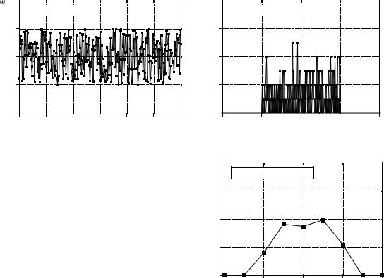
Example of binned histograms. As shown in (a), the signal used in this example is 300 samples long, with each sample a floating point number uniformly distributed between 1 and 3. Figures (b) and (c) show binned histograms of this signal, using 601 and 9 bins, respectively. As shown, a large number of bins results in poor resolution along the vertical axis, while a small number of bins provides poor resolution along the horizontal axis. Using more samples makes the resolution better in both directions.
|
160 |
|
|
|
|
occurences |
|
c. Histogram of 9 bins |
|
|
|
120 |
|
|
|
|
|
|
|
|
|
|
|
Number of |
80 |
|
|
|
|
40 |
|
|
|
|
|
|
0 |
|
|
|
|
|
0 |
2 |
4 |
6 |
8 |
Bin number in histogram
How many bins should be used? This is a compromise between two problems. As shown in Fig. 2-7, too many bins makes it difficult to estimate the amplitude of the underlying pmf. This is because only a few samples fall into each bin, making the statistical noise very high. At the other extreme, too few of bins makes it difficult to estimate the underlying pmf in the horizontal direction. In other words, the number of bins controls a tradeoff between resolution along the y-axis, and resolution along the x-axis.
The Normal Distribution
Signals formed from random processes usually have a bell shaped pdf. This is called a normal distribution, a Gauss distribution, or a Gaussian, after the great German mathematician, Karl Friedrich Gauss (1777-1855). The reason why this curve occurs so frequently in nature will be discussed shortly in conjunction with digital noise generation. The basic shape of the curve is generated from a negative squared exponent:
y (x ) ' e & x 2
Chapter 2- Statistics, Probability and Noise |
27 |
This raw curve can be converted into the complete Gaussian by adding an adjustable mean, µ, and standard deviation, F. In addition, the equation must be normalized so that the total area under the curve is equal to one, a requirement of all probability distribution functions. This results in the general form of the normal distribution, one of the most important relations in statistics and probability:
EQUATION 2-8
Equation for the normal distribution, also called the Gauss distribution, or simply a Gaussian. In this relation, P(x) is the probability distribution function, µ is the mean, and σ is the standard deviation.
P (x ) ' 1 e & (x & µ )2 /2F2
 2BF
2BF
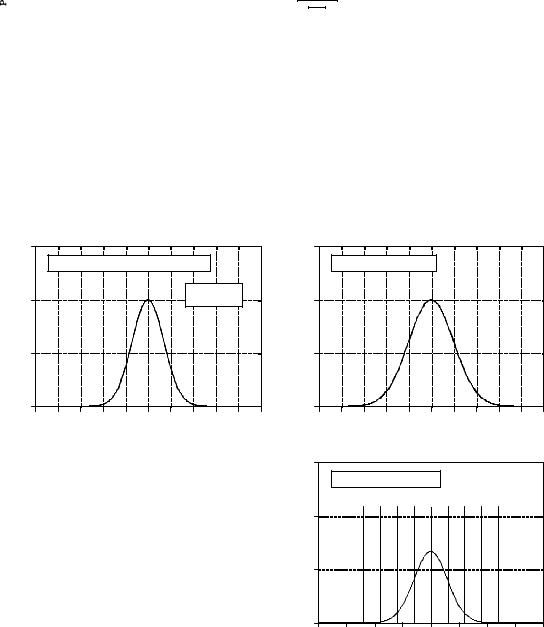
Figure 2-8 shows several examples of Gaussian curves with various means and standard deviations. The mean centers the curve over a particular value, while the standard deviation controls the width of the bell shape.
An interesting characteristic of the Gaussian is that the tails drop toward zero very rapidly, much faster than with other common functions such as decaying exponentials or 1/x. For example, at two, four, and six standard
1.5 |
|
|
|
|
|
|
|
|
|
|
|
a. Raw shape, no normalization |
|
|
|
||||||
1.0 |
|
|
|
|
|
|
y (x ) ' e & x 2 |
|
||
|
|
|
|
|
|
|
|
|
|
|
y(x) |
|
|
|
|
|
|
|
|
|
|
0.5 |
|
|
|
|
|
|
|
|
|
|
0.0 |
|
|
|
|
|
|
|
|
|
|
-5 |
-4 |
-3 |
-2 |
-1 |
0 |
1 |
2 |
3 |
4 |
5 |
|
|
|
|
|
x |
|
|
|
|
|
FIGURE 2-8
Examples of Gaussian curves. Figure (a) shows the shape of the raw curve without normalization or the addition of adjustable parameters. In (b) and (c), the complete Gaussian curve is shown for various means and standard deviations.
0.6 |
|
|
|
|
|
|
|
|
|
|
|
b. Mean = 0, F = 1 |
|
|
|
|
|
|
|||
0.4 |
|
|
|
|
|
|
|
|
|
|
P(x) |
|
|
|
|
|
|
|
|
|
|
0.2 |
|
|
|
|
|
|
|
|
|
|
0.0 |
|
|
|
|
|
|
|
|
|
|
-5 |
-4 |
-3 |
-2 |
-1 |
0 |
1 |
2 |
3 |
4 |
5 |
|
|
|
|
|
x |
|
|
|
|
|
0.3 |
|
|
|
|
|
|
|
|
|
|
|
c. Mean = 20, F = 3 |
|
|
|
|
|
||||
|
|
-4F -3F -2F -1F µ |
1F 2F 3F 4F |
|
|
|||||
0.2 |
|
|
|
|
|
|
|
|
|
|
P(x) |
|
|
|
|
|
|
|
|
|
|
0.1 |
|
|
|
|
|
|
|
|
|
|
0.0 |
|
|
|
|
|
|
|
|
|
|
0 |
5 |
10 |
|
15 |
20 |
25 |
|
30 |
35 |
40 |
|
|
|
|
|
x |
|
|
|
|
|

28 |
The Scientist and Engineer's Guide to Digital Signal Processing |
deviations from the mean, the value of the Gaussian curve has dropped to about 1/19, 1/7563, and 1/166,666,666, respectively. This is why normally distributed signals, such as illustrated in Fig. 2-6c, appear to have an approximate peak-to-peak value. In principle, signals of this type can experience excursions of unlimited amplitude. In practice, the sharp drop of the Gaussian pdf dictates that these extremes almost never occur. This results in the waveform having a relatively bounded appearance with an apparent peak- to-peak amplitude of about 6-8F.
As previously shown, the integral of the pdf is used to find the probability that a signal will be within a certain range of values. This makes the integral of the pdf important enough that it is given its own name, the cumulative distribution function (cdf). An especially obnoxious problem with the Gaussian is that it cannot be integrated using elementary methods. To get around this, the integral of the Gaussian can be calculated by numerical integration. This involves sampling the continuous Gaussian curve very finely, say, a few million points between -10F and +10F. The samples in this discrete signal are then added to simulate integration. The discrete curve resulting from this simulated integration is then stored in a table for use in calculating probabilities.
The cdf of the normal distribution is shown in Fig. 2-9, with its numeric values listed in Table 2-5. Since this curve is used so frequently in probability, it is given its own symbol: M(x) (upper case Greek phi). For example, M(&2) has a value of 0.0228. This indicates that there is a 2.28% probability that the value of the signal will be between -4 and two standard deviations below the mean, at any randomly chosen time. Likewise, the value: M(1) ' 0.8413 , means there is an 84.13% chance that the value of the signal, at a randomly selected instant, will be between -4 and one standard deviation above the mean. To calculate the probability that the signal will be will be between two values, it is necessary to subtract the appropriate numbers found in the M(x) table. For example, the probability that the value of the signal, at some randomly chosen time, will be between two standard deviations below the mean and one standard deviation above the mean, is given by: M(1) & M(&2) ' 0.8185 , or 81.85%
Using this method, samples taken from a normally distributed signal will be within ±1 F of the mean about 68% of the time. They will be within ±2 F about 95% of the time, and within ±3 F about 99.75% of the time. The probability of the signal being more than 10 standard deviations from the mean is so minuscule, it would be expected to occur for only a few microseconds since the beginning of the universe, about 10 billion years!
Equation 2-8 can also be used to express the probability mass function of normally distributed discrete signals. In this case, x is restricted to be one of the quantized levels that the signal can take on, such as one of the 4096 binary values exiting a 12 bit analog-to-digital converter. Ignore the 1/ 2BF term, it is only used to make the total area under the pdf curve equal to one. Instead, you must include whatever term is needed to make the sum of all the values in the pmf equal to one. In most cases, this is done by

Chapter 2- Statistics, Probability and Noise
 M(x)
M(x)
1.0
0.9 


0.8 


0.7 


0.6 


0.5 


0.4 


0.3 


0.2 


0.1 


0 |
|
|
|
|
|
|
|
|
|
|
|
|
|
|
|
|
|
|
|
|
|
-4 |
-3 |
-2 |
-1 |
0 |
1 |
2 |
3 |
4 |
|||||||||||||
|
|
|
|
|
|
|
|
|
|
|
x |
|
|
|
|
|
|
|
|
||
FIGURE 2-9 & TABLE 2-5
M(x), the cumulative distribution function of the normal distribution (mean = 0, standard deviation = 1). These values are calculated by numerically integrating the normal distribution shown in Fig. 2-8b. In words, M(x) is the probability that the value of a normally distributed signal, at some randomly chosen time, will be less than x. In this table, the value of x is expressed in units of standard deviations referenced to the mean.
x M(x)
-3.4 .0003 -3.3 .0005 -3.2 .0007 -3.1 .0010 -3.0 .0013 -2.9 .0019 -2.8 .0026 -2.7 .0035 -2.6 .0047 -2.5 .0062 -2.4 .0082 -2.3 .0107 -2.2 .0139 -2.1 .0179 -2.0 .0228 -1.9 .0287 -1.8 .0359 -1.7 .0446 -1.6 .0548 -1.5 .0668 -1.4 .0808 -1.3 .0968 -1.2 .1151 -1.1 .1357 -1.0 .1587 -0.9 .1841 -0.8 .2119 -0.7 .2420 -0.6 .2743 -0.5 .3085 -0.4 .3446 -0.3 .3821 -0.2 .4207 -0.1 .4602
0.0.5000
29
x M(x)
0.0.5000
0.1.5398
0.2.5793
0.3.6179
0.4.6554
0.5.6915
0.6.7257
0.7.7580
0.8.7881
0.9.8159
1.0.8413
1.1.8643
1.2.8849
1.3.9032
1.4.9192
1.5.9332
1.6.9452
1.7.9554
1.8.9641
1.9.9713
2.0.9772
2.1.9821
2.2.9861
2.3.9893
2.4.9918
2.5.9938
2.6.9953
2.7.9965
2.8.9974
2.9.9981
3.0.9987
3.1.9990
3.2.9993
3.3.9995
3.4.9997
generating the curve without worrying about normalization, summing all of the unnormalized values, and then dividing all of the values by the sum.
Digital Noise Generation
Random noise is an important topic in both electronics and DSP. For example, it limits how small of a signal an instrument can measure, the distance a radio system can communicate, and how much radiation is required to produce an x- ray image. A common need in DSP is to generate signals that resemble various types of random noise. This is required to test the performance of algorithms that must work in the presence of noise.
The heart of digital noise generation is the random number generator. Most programming languages have this as a standard function. The BASIC statement: X = RND, loads the variable, X, with a new random number each time the command is encountered. Each random number has a value between zero and one, with an equal probability of being anywhere between these two extremes. Figure 2-10a shows a signal formed by taking 128 samples from this type of random number generator. The mean of the underlying process that generated this signal is 0.5, the standard deviation is 1 / 12 ' 0.29 , and the distribution is uniform between zero and one.

30 |
The Scientist and Engineer's Guide to Digital Signal Processing |
Algorithms need to be tested using the same kind of data they will encounter in actual operation. This creates the need to generate digital noise with a Gaussian pdf. There are two methods for generating such signals using a random number generator. Figure 2-10 illustrates the first method. Figure (b) shows a signal obtained by adding two random numbers to form each sample, i.e., X = RND+RND. Since each of the random numbers can run from zero to one, the sum can run from zero to two. The mean is now one, and the standard deviation is 1 / 6 (remember, when independent random signals are added, the variances also add). As shown, the pdf has changed from a uniform d i s t r i b u t i o n t o a triangular distribution. That is, the signal spends more of its time around a value of one, with less time spent near zero or two.
Figure (c) takes this idea a step further by adding twelve random numbers to produce each sample. The mean is now six, and the standard deviation is one. What is most important, the pdf has virtually become a Gaussian. This procedure can be used to create a normally distributed noise signal with an arbitrary mean and standard deviation. For each sample in the signal: (1) add twelve random numbers, (2) subtract six to make the mean equal to zero, (3) multiply by the standard deviation desired, and (4) add the desired mean.
The mathematical basis for this algorithm is contained in the Central Limit Theorem, one of the most important concepts in probability. In its simplest form, the Central Limit Theorem states that a sum of random numbers becomes normally distributed as more and more of the random numbers are added together. The Central Limit Theorem does not require the individual random numbers be from any particular distribution, or even that the random numbers be from the same distribution. The Central Limit Theorem provides the reason why normally distributed signals are seen so widely in nature. Whenever many different random forces are interacting, the resulting pdf becomes a Gaussian.
In the second method for generating normally distributed random numbers, the random number generator is invoked twice, to obtain R1 and R2. A normally distributed random number, X, can then be found:
EQUATION 2-9 |
|
|
|
|
|
|
Generation of normally distributed random |
|
|
|
|
|
|
numbers. R1 and R2 are random numbers |
|
|
|
|
|
|
with a uniform distribution between zero and |
X ' (& 2 log R |
1 |
)1/2 |
cos(2BR |
2 |
) |
one. This results in X being normally |
|
|
|
|
distributed with a mean of zero, and a standard deviation of one. The log is base e, and the cosine is in radians.
Just as before, this approach can generate normally distributed random signals with an arbitrary mean and standard deviation. Take each number generated by this equation, multiply it by the desired standard deviation, and add the desired mean.