Потоковые методы

Previously we developed our differencing schemes by considering Taylor series expansions about a point. In this section, we will develop an alternative approach for deriving difference equations that is similar to the way we developed the original conservation equations. This approach will become useful for deriving the upwind and mpdata schemes described below.

The control volume approach divides up space into a number of control volumes of width _x surrounding each node i.e. and then considers the integral form of the conservation equations

If we now consider that the value of c at the center node of volume j is representative of the average value of the control volume, then we can replace the first integral by cj_x. The second integral is the surface integral of the flux and is exactly

which is just the difference between the flux at the boundaries Fj+1/2 and Fj−1/2.

Figure: A simple staggered grid used to define the control volume approach. Dots denote nodes where average values of the control volume are stored. X’s mark control volume boundaries at half grid points.

If we assume that we can interpolate linearly between nodes then cj+1/2 = (cj+1 +cj)/2. If we use a centered time step for the time derivative then the flux conservative centered approximation to

or if V is constant Eq. (5.5.13) reduces identically to the staggered leapfrog scheme. By using higher order interpolations for the fluxes at the boundaries additional differencing schemes are readily derived. The principal utility of this sort of differencing scheme is that it is automatically flux conservative as by symmetry what leaves one box must enter the next. The following section will develop a slightly different approach to choosing the fluxes by the direction of transport.

Численная схема против потока (донорская ячейка)

The fundamental behavior of transport equations such as (5.5.13) is that every particle will travel at its own velocity independent of neighboring particles (remember the characteristics), thus physically it might seem more correct to say that if the flux is moving from cell j − 1 to cell j the incoming flux should only depend on the concentration upstream. i.e. for the fluxes shown in Fig. 5.6 the upwind differencing for the flux at point j − 1/2 should be

with a similar equation for Fj+1/2. Thus the concentration of the incoming flux is determined by the concentration of the donor cell and thus the name. As a note, the donor cell selection can be coded up without an if statement by using the following trick

Simple upwind donor-cell schemes are stable as long as the Courant condition is met. Unfortunately they are only first order schemes in _t and _x and thus the truncation error is second order producing large numerical diffusion (it is this diffusion which stabilizes the scheme). If we do a Hirt’s style stability analysis for constant velocities, we find that the actual equations being solved to second order

are

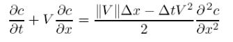
or in terms of the Courant number

Thus as long as _ < 1 this scheme will have positive diffusion and be stable. Unfortunately, any initial feature won’t last very long with this much diffusion. Figure (5.7) shows the effects of this scheme on a long run with a gaussian initial condition. The boundary conditions for this problem are periodic (wraparound) and thus every new curve marks another pass around the grid (i.e. after t = 10 the peak should return to its original position). A staggered leapfrog solution of this problem would be almost indistinguishable from a single gaussian.