Методы решения уравнения переноса газов в адвективной форме

Адвективный перенос газовых примесей описывается дифференциальным уравнением в частных производных, в предположении расщепления системы уравнений баланса по процессам в потоковой форме

где - концентрации вычисляемых газов,-зональная, меридиональная и вертикальная компоненты скорости ветра,- число вычисляемых газов.

Аналогичная система уравнений в адвективной форме может быть записана для отношений смеси

где - отношения смеси вычисляемых газов.

Так как, в результате применения метода расщепления, связи между уравнениями нет, т.е. исходная система потеряла жесткость, уравнения можно решать по отдельности для каждой газовой компоненты и использовать для этого стандартные методы решения уравнения адвекции.

Численные методы решения уравнения адвекции

The basic idea behind Finite-difference, grid-based methods is to slap a static grid over the solution space and to approximate the partial differentials at each point in the grid. The standard approach for approximating the differentials comes from truncated Taylors series. Consider a function f(x, t) at a fixed time t. If f is continuous in space we can expand it around any point f(x + _x) as

where the subscripted x imply partial differentiation with respect to x. If we ignore terms in this series of order _x² and higher we could approximate the first derivative at any point x₀ as

If we consider our function is now stored in a discrete array of points fj and x = _xj where _x is the grid spacing, then at time step n we can write the forward space or FS derivative as

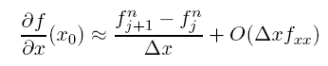
An identical procedure but expanding in time gives the forward time derivative (FT) as

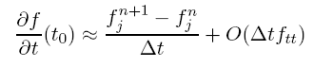
Both of these approximations however are only first order accurate as the leading term in the truncation error is of order _x or _t. More importantly, this approximation will only be exact for piecewise linear functions where fxx or ftt = 0.

Other combinations and higher order schemes In Eq. (5.3.1) we considered the value of our function at one grid point forward in _x. We could just have easily taken a step backwards to get

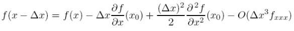
If we truncate at order _x2 and above we still get a first order approximation for the Backward space step (BS)

which isn’t really any better than the forward step as it has the same order error (but of opposite sign). We can do a fair bit better however if we combine Eqs. (5.3.1) and (5.3.5) to remove the equal but opposite 2nd order terms. If we subtract (5.3.5) from (5.3.1) and rearrange, we can get the centered space (CS) approximation

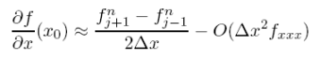
Note we have still only used two grid points to approximate the derivative but have gained an order in the truncation error. By including more and more neighboring points, even higher order schemes can be dreamt up (much like the 4th order Runge Kutta ODE scheme), however, the problem of dealing with large patches of points can become bothersome, particularly at boundaries. By the way, we don’t have to stop at the first derivative but we can also come up with approximations for the second derivative (which we will need shortly). This time, by adding (5.3.1) and (5.3.5) and rearranging we get

This form only needs a point and its two nearest neighbours. Note that while the truncation error is of order _x2 it is actually a 3rd order scheme because a cubic polynomial would satisfy it exactly (i.e. fxxxx = 0).