

0303014
.pdfYu.I. Bogdanov LANL Report quant-ph/0303014 |
|
(n + m)= λ1 +λ2 E . |
(2.9) |
The sample mean energy E (i.e., the sum of the mean potential energy that can be measured in the coordinate space and the mean kinetic energy measured in the momentum space) was used as the estimator of the mean energy in numerical simulations below.
Now, let us turn to the study of statistical fluctuations of a state vector in the problem under consideration. We restrict our consideration to the energy representation in the case when the expansion basis is formed by stationary energy states (that are assumed to be nondegenerate).
Additional condition (2.3) related to the conservation of energy results in the following relationship between the components
δ |
|
=∑s−1 |
(Ejcjδcj +Ejδcjcj )=0. |
|
E |
(2.10) |
|||
|
|
j=0 |
|
|
It turns out that both parts of the equality can be reduced to zero independently if one assumes that a state vector to be estimated involves a time uncertainty, i.e., may differ from the true one by a small time translation. The possibility of such a translation is related to the time-energy uncertainty relation.
The well-known expansion of the psi function in terms of stationary energy states, in view
of time dependence, has the form ( h =1) |
|
ψ(x)= ∑cj exp(−iEj (t −t0 ))ϕj (x)= |
|
j |
|
= ∑cj exp(iEjt0 )exp(−iEjt)ϕj (x) |
(2.11) |
|
|
j |
|
In the case of estimating the state vector up to translation in time, the transformation |
|
c′j = cj exp(iEjt0 ) |
(2.12) |
related to arbitrariness of zero-time reference t0 may be used to fit the estimated state vector to the
true one.
The corresponding infinitesimal time translation leads us to the following variation of a state
vector: |
|
δcj =it0Ejcj . |
(2.13) |
Let δc be any variation meeting both the normalization condition and the law of energy |
|
conservation. Then, from (1.15) and (2.3) it follows that |
|
∑(δcj )cj =iε1 , |
(2.14) |
j |
|
∑(δcj )Ejcj =iε2 , |
(2.15) |
j |
|
where ε1 and ε2 are arbitrary small real numbers. |
|
In analogy with Sec.1, we divide the total variation δc into |
unavoidable physical |
fluctuation δ2c and variations caused by the gauge and time invariances: |
|
δcj =iαcj +it0Ejcj +δ2cj . |
(2.16) |
11
Yu.I. Bogdanov LANL Report quant-ph/0303014
We will separate out the physical variation δ2c , so that it fulfills the conditions (2.14) and
(2.15) with a zero right part. It is possible if the transformation parameters α and |
t0 satisfy the |
|||||||||||||||
following set of linear equations: |
|
|||||||||||||||
|
α + |
|
|
|
|
|
=ε |
|
|
|
||||||
Et |
0 |
1 |
|
|||||||||||||
|
|
|
|
|
|
|
|
|
|
|
|
|
|
|
||
|
|
|
|
|
|
|
|
|
|
|
|
|
|
|
. |
(2.17) |
|
|
|
|
|
|
|
|
|
|
|
|
|
|
|
||
Eα + E |
2 |
t0 =ε2 |
|
|
||||||||||||
|
|
|||||||||||||||
|
|
|
|
|
|
|
|
|
|
|
|
|
|
|||
The determinant of (2.17) is the energy variance |
|
|||||||||||||||
|
|
|
|
|
||||||||||||
σE2 = |
E2 |
− |
|
2 . |
|
|
||||||||||
E |
|
(2.18) |
||||||||||||||
We assume that the energy variance is a positive number. Then, there exists a unique solution of the set (2.17). If the energy dissipation is equal to zero, the state vector has the only nonzero component. In this case, the gauge transformation and time translation are dependent, since they are reduced to a simple phase shift.
In full analogy with the reasoning on the gauge invariance, one can show that in view of both the gauge invariance and time homogeneity, the transformation satisfying (2.17) provides minimization of the total variance of the variations (sum of squares of the components absolute values). Thus, one may infer that physical fluctuations are minimum possible fluctuations compatible with the conservation of norm and energy.
Let us make an additional remark about the time translation introduced above. We will estimate the deviation between the estimated and exact state vectors by the difference between their scalar product and unity. Then, one can state that the estimated state vector is closest to the true one specified in the time instant that differs from the “true” one by a random quantity. In other words, a quantum ensemble can be considered as a time meter, statistical clock, measuring time within the accuracy up to the statistical fluctuation asymptotically tending to zero with increasing number of particles of the system. Time measurement implies the comparison between the readings of real and reference systems. The dynamics of the state vector of a reference system corresponds to an infinite ensemble and is determined by the solution of the Schrödinger equation. The estimated state vector of a real finite system is compared with the “world-line” of an ideal vector in the Hilbert space, and the time instant when the ideal vector is closest to the real one is considered as the reading of the statistical clock. Note that ordinary clock operates in the similar way: their readings correspond to the situation when the scalar product of the real vector of a clock hand and the reference one making one complete revolution per hour reaches maximum value.
|
Assuming that the total variations are reduced to the physical ones, we assume hereafter that |
|||||
|
∑(δcj )cj = 0, |
(2.19) |
||||
|
|
j |
|
|
|
|
|
∑(δcj )Ejcj = 0. |
(2.20) |
||||
|
|
j |
|
|
|
|
|
The relationships found yield (in analogy with Sec.1) the conditions for the covariance |
|||||
|
|
|
|
|
||
matrix |
Σ |
ij |
= |
δc δc |
|
|
|
|
i j : |
|
|||
|
∑(Σijcj )= 0 , |
(2.21) |
||||
|
|
j |
|
|
|
|
|
∑(Σij Ejcj )= 0 . |
(2.22) |
||||
|
|
j |
|
|
|
|
|
Consider the unitary matrix U + |
with the following two rows (zero and first): |
||||
12
Yu.I. Bogdanov LANL Report quant-ph/0303014
(U + ) |
|
= c |
|
|
(2.23) |
|||
0 j |
|
j , |
|
|
||||
(U + ) |
|
|
(Ej − |
|
)cj |
|
|
|
= |
E |
j =0,1,...,s −1 |
. |
(2.24) |
||||
|
|
|
|
|||||
1 j |
|
|
σE |
|
||||
|
|
|
|
|
|
|||
This matrix determines the transition to principle components of the variation |
|
|||||||
Uij+δcj |
=δfi . |
|
|
(2.25) |
||||
According to (2.19) and (2.20), we have δf0 =δf1 = 0 identically in new variables so
that there remain only s −2 independent degrees of freedom. The inverse transformation is
Uδf =δc . |
|
|
|
|
(2.26) |
|||
On account of the fact that δf0 =δf1 = 0, one may drop two columns (zero and first) in |
||||||||
the U matrix turning it into the factor loadings matrix L |
|
|||||||
Lijδf j =δci |
i = 0,1,...,s −1; j = 2,3,...,s −1. |
(2.27) |
||||||
The L matrix has s rows and |
s −2 columns. Therefore, it provides the transition from s −2 |
|||||||
independent variation principle components to s components of the initial variation. |
|
|||||||
In principal components, the Fisher information matrix and covariance matrix are given by |
||||||||
Iijf |
= (n +m)δij , |
|
|
|
(2.28) |
|||
|
|
|
|
(n +m) |
|
|
||
|
|
|
|
|
|
|||
Σijf |
=δfiδf j = |
1 |
|
|
δij . |
(2.29) |
||
|
|
|
||||||
In order to find the covariance matrix for the state vector components, we will take into
account the fact that the factor loadings matrix |
|
|
L differs form the unitary matrix |
|||||||||||||||||||||||||||
absence of two aforementioned columns, and hence, |
|
|
||||||||||||||||||||||||||||
L L+ =δ −c c − |
(Ei − |
|
)(Ej − |
|
) |
|
c c |
|
||||||||||||||||||||||
E |
E |
, |
||||||||||||||||||||||||||||
|
|
|
σ2 |
|
|
|
|
|
|
|
|
|||||||||||||||||||
|
ik |
kj |
|
ij |
|
|
i |
j |
|
|
|
|
|
|
|
|
|
|
|
|
i |
j |
||||||||
|
|
|
|
|
|
|
|
|
|
|
|
|
|
|
|
|
|
|
|
|||||||||||
|
|
|
|
|
|
|
|
|
|
|
|
|
|
|
E |
|
|
|
|
|
|
|
|
|
|
|
|
|
|
|
|
|
|
|
|
|
|
|
|
|
|
|
|
|
|
|
|
|
|
|
L L+ |
|
|
||||||||
|
|
|
|
|
|
|
|
|
|
|
|
|
|
|
|
|
|
|
|
|
|
|||||||||
Σ =δc δc = L L δf δf |
= |
ik kj |
|
|
|
|||||||||||||||||||||||||
n |
+m . |
|
|
|||||||||||||||||||||||||||
|
ij |
|
|
i |
|
j |
|
ik jr |
k |
r |
|
|
|
|
|
|||||||||||||||
|
|
|
|
|
|
|
|
|
|
|
|
|
|
|
|
|
|
|
||||||||||||
Finally, the covariance matrix in the energy representation takes the form |
||||||||||||||||||||||||||||||
|
|
|
|
|
|
|
|
|
|
|
(E |
− |
|
)(E |
|
|
− |
|
) |
|||||||||||
|
|
|
|
1 |
|
|
|
E |
j |
E |
||||||||||||||||||||
Σ |
|
= |
|
|
δ |
|
−c c 1+ |
|
|
i |
|
|
|
|
|
|
|
|
|
|
|
|
|
|||||||
|
|
|
|
|
|
|
|
|
|
|
σ 2 |
|
|
|
|
|
|
|
|
|||||||||||
|
ij |
|
(n +m) |
ij |
i j |
|
|
|
|
|
|
|
|
|
|
|
|
|
|
|
||||||||||
|
|
|
|
|
|
|
|
|
|
|
|
|
|
|
|
|
|
E |
|
|
|
|
|
|
|
|
. |
|||
i, j = 0,1,...,s −1
U by the
(2.30)
(2.31)
(2.32)
It is easily verified that this matrix satisfies the conditions (2.21) and (2.22) resulting from the conservation of norm and energy.
The mean square fluctuation of the psi function is
∫ |
|
dx = ∫ |
|
|
|
|
s −2 |
|
|
δψδψ |
δciϕi (x)δcjϕj (x)dx =δciδci =Tr(Σ)= |
. (2.33) |
|||||||
n +m |
|||||||||
|
|
|
|
|
|
|
|
||
13
Yu.I. Bogdanov LANL Report |
quant-ph/0303014 |
|
|||||||
The estimation of optimal number of harmonics in the Fourier series, similar to that in Sec.6 |
|||||||||
of the Paper.1, has the form |
|
|
|
|
|||||
s |
= r +1 rf (n + m) |
, |
(2.34) |
||||||
opt |
|
|
|||||||
where the parameters r and |
f |
|
determine the asymptotics for the sum of squares of residuals: |
||||||
|
∞ |
f |
|
|
|
||||
Q(s)= ∑ |
|
ci |
|
2 = |
|
. |
(2.35) |
||
|
|
|
|||||||
|
|
r |
|
||||||
|
i=s |
s |
|
|
|
||||
The norm existence implies only that r > 0 . In the case of statistical ensemble of harmonic
oscillators with existing energy, r >1. If the energy variance is defined as well, r > 2.
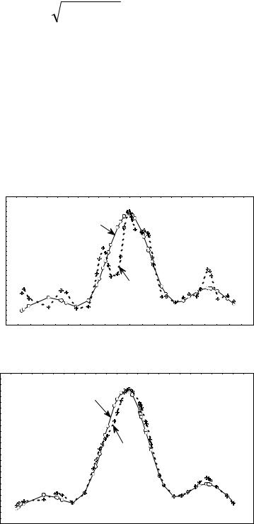
Figure 4 shows how the constraint on energy decreases high-energy noise. The momentumspace density estimator disregarding the constraint on energy (upper plot) is compared to that accounting for the constraint.
Fig. 4 (a) An estimator without the constraint on energy;
(b) An estimator with the constraint on energy.
P(p)
0,6 a)
s=3
0,5
0,4
0,3
0,2 |
s=100 |
0,1 |
|
0,0
-2 |
-1 |
0 |
1 |
2 |
p
P(p)
0,6 |
b) |
0,5 |
s=3 |
|
|
0,4 |
|
0,3 |
s=100 |
0,2
0,1
0,0
-2 |
-1 |
0 |
1 |
2 |
p
The sample of the size of n = m =50 ( n +m =100) was taken from the statistical ensemble of harmonic oscillators. The state vector of the ensemble had three nonzero components ( s =3).
Figure 4 shows the calculation results in bases involving s =3 and functions, respectively. In the latter case, the number of basis functions coincided with the total sample size. Figure 4 shows that in the case when the constraint on energy was taken into account, the 97 additional noise components influenced the result much weaker than in the case without the constraint.
14
Yu.I. Bogdanov LANL Report quant-ph/0303014
3. Spin State Reconstruction
The aim of this section is to show the application of the approach developed above to reconstruct spin states (by an example of the ensemble of spin-1/2 particles).
We will look for the state vector in the spinor form
|
1 |
|
0 |
c |
|
|
|
|
|
|
|
|
1 |
|
|
|
|
ψ =c1 |
0 +c2 |
1 |
= c |
|
|
(3.1) |
|
|
|
|
|
|
2 |
|
|
|
|
The spin projection operator to direction nr is |
|
|
||||||
P(s =±1/ 2)= |
1 (1±σrnr) |
|
(3.2) |
|
||||
n |
r |
2 |
|
|
|
|
||
|
|
|
|
|
|
|||
We will set n by the spherical angles |
|
|
||||||
nr = (nx , ny , nz )= (sinθ cosϕ, sinθ sin ϕ, cosθ ) |
(3.3) |
r |
||||||
The probabilities |
for |
a particle to |
have positive and negative projections along the n |
|||||
direction are |
|
|
|
|
|
|
|
|
P (nr)= 1 ψ P(s =+1/ 2)ψ = 1 ψ 1+σrnrψ |
(3.4) |
|
||||||
+ |
2 |
|
n |
|
|
2 |
|
|
|
|
|
|
|
|
|
||
P (nr)= 1 ψ P(s =−1/ 2)ψ = |
1 ψ 1−σrnrψ |
(3.5) |
|
|||||
− |
2 |
|
n |
|
|
2 |
|
|
|
|
|
|
|
|
|
||
respectively.
Direct calculation yields the following expressions for the probabilities under consideration:
P+(nr)=P+(θ,ϕ)= 12[(1+cosθ)c1*c1 +sinθ e−iϕc1*c2 +sinθ eiϕc2*c1 +(1−cosθ)c2*c2 ] (3.6)
P−(nr)= P−(θ,ϕ)= 12[(1−cosθ)c1*c1 −sinθ e−iϕc1*c2 −sinθ eiϕc2*c1 +(1+cosθ)c2*c2 ] (3.7)
|
These probabilities evidently satisfy the condition |
|
|
|
P+(θ,ϕ)+P−(θ,ϕ)=1 |
(3.8) |
|
|
The likelihood function is given by the following product over all the directions involved in |
||
measurements: |
|
|
|
|
L =∏(P+(nr))N+(nr)(P−(nr))N−(nr) |
(3.9) |
|
|
r |
|
|
Here, N+(nr) andn |
N−(nr) are the numbers of spins with positive and negative projections along |
||
the nr |
direction. In order to reconstruct the state vector of a particle, one |
has to conduct |
|
measurements at least in three noncomplanar (linearly independent) directions. |
|
||
The total number of measurements is |
|
||
|
N =∑N(nr)=∑(N+(nr)+N−(nr)) |
(3.10) |
|
|
nv |
nv |
|
15
Yu.I. Bogdanov LANL Report quant-ph/0303014
In complete analogy to (1.8), we will find the likelihood equation represented by the set of two equations in two unknown complex numbers c1 and c2 .
1 |
|
|
r |
|
|
|
−iϕ |
|
r |
|
|
|
|
|
−iϕ |
|
|
|
|
|||||
∑ |
N+ (rn) |
[(1 |
+ cosθ )c1 +sinθe |
|
c2 ]+ |
N− (rn) |
[(1 |
−cosθ )c1 −sinθe |
|
|
c2 |
] |
= c1 |
(3.11) |
||||||||||
N |
|
|
|
|||||||||||||||||||||
nr |
|
P+ (n) |
|
|
2 |
|
|
P− (n) |
|
|
|
2 |
|
|
|
|
|
|
|
|||||
1 |
|
|
r |
|
iϕ |
|
|
|
r |
|
iϕ |
|
|
|
|
|
|
|
|
|
||||
|
|
|
|
|
|
|
|
|
|
|
|
|
|
|
|
|
|
|
|
|
|
|||
∑ |
N+ (rn) |
[ sinθe |
|
c1 + (1−cosθ )c2 ]+ |
N− (rn) |
[−sinθe |
|
c1 + (1+ cosθ )c2 ] |
= c2 |
(3.12) |
||||||||||||||
N |
|
|
||||||||||||||||||||||
nr |
|
P+ (n) |
|
|
2 |
|
|
P− (n) |
P (nr) |
2 |
P (nr) |
|
|
|
|
|
||||||||
|
|
This system is nonlinear, since the probabilities |
and |
depend on the unknown |
||||||||||||||||||||
|
|
+ |
|
|
− |
|
||||||||||||||||||
amplitudes c1 and c2 .
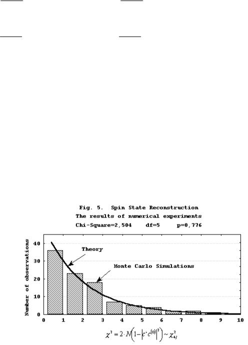
This system can be easily solved by the method of iterations. The resultant estimated state vector will differ from the true state vector by an asymptotically small random number (the squared absolute value of the scalar product of the true and estimated vectors is close to unity). The corresponding asymptotical formula has the form
|
|
|
+ |
(0) |
|
2 |
~2 |
χ42j |
|
|
|
|
|||||||
N 1− |
|
c c |
|
|
|
=χ2 j = |
|
(3.13) |
|
|
|
|
|
||||||
|
|
|
|
|
|
|
|
2 |
|
|
|
|
|
|
|
||||
Here, χ42j |
is the random number with the chi-square distribution of 4 j degrees of freedom, |
||||||||
and j is the particle spin ( j =1/ 2 in our case).
The validity of the formula (3.13) is illustrated with Fig. 5. In this figure, the results of 100
numerical experiments are presented. In each experiment, the spin j =1/ 2 of a pure ensemble has been measured along 200 random space directions by 50 particles in each direction, i.e.,
N =200 50=10000. In this case, the left side of (3.13) is the half of a random variable with the chi-square distribution of 4j =2 degrees of freedom.
16
Yu.I. Bogdanov LANL Report quant-ph/0303014
Incoherent mixture is described in the framework of the density matrix. Two samples are referred to as mutually incoherent if the squared absolute value of the scalar product of their state vector estimates is statistically significantly different from unity. The quantitative criterion is
|
|
N N |
|
|
|
+(1) (2) |
|
2 |
|
|
2 |
|
χα2,4 j |
|
|
|
|||
|
|
|
|
|
|
|
|
|
|
||||||||||
|
1 |
2 |
|
c |
|
c |
|
|
~ |
|
|
|
|
|
|
||||
|
|
|
|
1− |
|
|
|
>χ |
|
= |
|
|
|
|
|
||||
|
|
|
|
|
|
|
|
|
|
|
|||||||||
|
|
N +N |
|
|
|
|
|
|
|
|
α,2 j |
|
2 |
|
|
|
(3.14) |
||
|
1 |
2 |
|
|
|
|
|
|
|
|
|
|
|
|
|
|
|
||
|
Here, |
N and |
N |
are the sample sizes, and |
χ2 |
|
is the quantile corresponding to the |
||||||||||||
|
|
|
1 |
|
|
|
2 |
|
|
|
|
|
|
|
|
|
α,2 j |
|
|
significance level α for the chi-square distribution of |
2 j |
|
degrees of freedom. The significance |
||||||||||||||||
level |
α describes the probability of error of the first kind, i.e., the probability to find samples |
||||||||||||||||||
inhomogeneous while they are homogeneous (described by the same psi function). |
|||||||||||||||||||
|
Let us |
outline |
the |
process |
of |
reconstructing states |
with arbitrary spin. Let ψm(j) be the |
||||||||||||
amplitude of the probability to have the projection m along the z axis in the initial coordinate
frame (these |
are |
|
the |
quantities to be estimated |
by the results of |
measurements), |
|||||
|
|
|
|
|
~ |
|
|
|
|
|
|
|
|
|
|
|
(j) |
be the corresponding quantities in the rotated coordinate frame. |
|||||
m=( j, j −1,...,−j). Let ψm |
|||||||||||
|
|
|
|
|
|
|
|
(j) |
|
2 |
|
|
|
|
|
|
|
|
|
|
|
||
The probability to get the value m in measurement along the z′ axis is |
~ |
|
. |
|
|||||||
ψm |
|
|
|||||||||
Both rotated and initial amplitudes are related to each other by the unitary transformation |
|||||||||||
|
(j) |
|
*(j) |
(j) |
|
|
|
|
|
|
|
~ |
=D |
′ψ ′ |
|
|
|
|
|
|
|||
ψ |
m |
|
|
|
|
|
(3.15) |
||||
|
|
mm |
m |
|
D(j)′(α,β,γ) |
||||||
The matrix |
D(j)′ |
is a function of the Euler angles |
, where the angles |
||||||||
|
mm |
mm |
|||||||||
α and β coincide with the spherical angles of the z′ axis with respect to the initial coordinate frame xyz, so that α =ϕ and β =θ . The angle γ corresponds to the additional rotation of the coordinate frame with respect to the z′ axis (this rotation is insignificant in measuring the spin
projection along the z′ axis, and it can be set γ =0). The matrix Dm(jm)′ is described in detail in
[14]. Note that our transformation matrix in (3.15) corresponds to the inverse transformation with respect to that considered in [14].
|
The likelihood equation in this case has the form |
|
|
|
|||||||||||
|
1 |
|
∑ |
N ′(ϕ,θ)D(j′) |
(ϕ,θ) |
(j) |
|
|
|
||||||
|
|
|
|
|
m |
*(j) |
|
|
=ψm |
|
|
|
|||
|
|
|
|
|
|
|
|
m m |
|
|
|
|
|
|
|
|
|
N |
′ ϕ θ |
|
|
ψ |
|
|
|
|
|
, |
|
(3.16) |
|
|
|
|
m , , |
|
|
~ |
′ |
|
|
|
|
|
|||
|
|
|
|
(ϕ,θ) |
|
m |
|
|
|
|
′ |
|
|
||
where |
N |
|
|
|
|
|
|
|
|
′ |
|||||
|
m′ |
|
|
is the number of spins with the projection m along the |
z |
axis with |
|||||||||
direction determined by the spherical angles ϕ and θ, and N is the total number of measured spins.
4. Mixture Division
There are two different methods for constructing the likelihood function for a mixture resulting in two different ways to estimate the density (density matrix). In the first method (widely
17
Yu.I. Bogdanov LANL Report quant-ph/0303014
used in problems of estimating quantum states [7-10]), the likelihood function for the mixture is constructed regardless a mixed (inhomogeneous) data structure (structureless approach). In this case, for the two-component mixture, we have
L0 |
= ∏n |
p(xi |
|
c(1),c(2), f1 , f2 ), |
(4.1) |
|
|||||
|
i=1 |
|
|
|
|
where the mixture density is given by |
|
||||
p(x)= f1 p1 (x)+ f2 p2 (x); |
(4.2) |
||||
p1 (x) and |
p2 (x) are the densities of the mixture components; f1 |
and f2 , their weights. |
|||
The normalization condition is |
|
||||
f1 + f2 =1 |
(4.3) |
||||
Here, it is assumed that all the points of the mixed sample |
xi ( i =1,2,..., n ) are taken from |
||||
the same |
distribution p(x)= f1 p1 (x)+ f2 p2 (x). In other |
words, the mixture of two |
|||
inhomogeneous samples (i.e., taken from two different distributions) is treated as a homogeneous sample taken from an averaged distribution.
The second approach, which seems to be more physically adequate, is based on the notion of a mixture as an inhomogeneous population (component approach). This implies that the mixed
sample is considered as an |
inhomogeneous population with n1 ≈ f1n points taken from the |
distribution with the density |
p1 (x) and the other n2 ≈ f2 n points, from the distribution with the |
density p2 (x). |
|
This approach has also formal advantages compared to the first one: it provides higher value of the likelihood function (and hence, higher value of information); besides that, basic theory structures, such as the Fisher information matrix and covariance matrix, take a block form. Thus, the problem is reduced to the division of an inhomogeneous (mixed) population into homogeneous (pure) sub-populations.
In view of the mixed data structure, the likelihood function in the component approach is given by
L1 = ∏n1 |
p1 (xi |
|
c(1))∏n |
p2 (xi |
|
c(2)). |
(4.4) |
|
|
||||||
i=1 |
|
|
i=n1 +1 |
|
|
|
|
Two different cases are possible:
1- population is divided into components a priory from the physical considerations (for instance, n1 values are taken from one source and n2 , from another source)
2- dividing the population into components have to be done on the basis of data itself without any information about sources (“blindly”)
The first case does not present difficulties, since it is reduced to analyzing homogeneous components in turn. The case when prior information about the sources is lacking requires additional considerations. In order to divide the mixture in this case, we will employ the so-called
randomized (mixed) strategy. In this approach, we will consider the observation xi to be taken |
|||||||||||||||||||||||||||||||
from the first distribution with the probability |
|
|
|
|
|
f1 p1 (xi ) |
|
|
|
|
; and from the second one, |
||||||||||||||||||||
|
f |
p |
(x |
i |
)+ f |
2 |
p |
2 |
(x |
i |
) |
||||||||||||||||||||
|
|
|
f2 p2 (xi ) |
|
|
|
|
|
|
|
|
|
|
|
1 1 |
|
|
|
|
|
|
|
|||||||||
|
|
|
|
|
|
|
. Having divided the sample into two population, we will find new estimates |
||||||||||||||||||||||||
|
f |
p |
(x |
i |
)+ f |
2 |
p |
2 |
(x |
i |
) |
||||||||||||||||||||
|
|
1 1 |
|
|
|
|
|
|
f = n1 |
|
|
|
|
|
|
|
|
|
|
|
|
|
|
|
|
|
|||||
of their weights by the formulas |
and |
f |
2 |
= |
n2 |
, as well as estimates of the state vectors for |
|||||||||||||||||||||||||
|
|||||||||||||||||||||||||||||||
1 |
n |
|
|
|
n |
|
|||||||||||||||||||||||||
|
|
|
|
|
|
|
|
|
|
|
|
|
|
|
|
|
|
|
|
|
|
|
|
|
|
|
|
|
|
||
18
Yu.I. Bogdanov LANL Report quant-ph/0303014
each population ( c(1) and c(2)) according to the algorithm presented above. Then, we will find the component densities
p |
|
(x)= |
|
c(1)ϕ |
(x) |
|
2 |
|||||||
|
|
|
||||||||||||
1 |
|
|
|
|
|
i |
i |
|
|
|
(4.5) |
|||
p |
2 |
(x)= |
|
c(2)ϕ |
(x) |
|
2 |
|||||||
|
|
|||||||||||||
|
|
|
|
|
i |
|
i |
|
|
(4.6) |
||||
Finally, instead of the initial (prior) estimates of the weights and densities, we will find new (posterior) weights and densities of the mixture components. Applying this (quasiBayesian) procedure repeatedly, we will arrive at a certain equilibrium state when the weights and densities of the components become approximately constant (more precisely, prior and posterior estimates of weights and densities become indistinguishable within statistical fluctuations).
A random-number generator should be used for numerical implementation of the algorithm proposed. Each iteration starts with the setting of the random vector of the length n from a homogeneous distribution on the segment [0,1]. If the same random vector is used at each iteration, the distribution of sample points between components will stop varying after some iterations, i.e., each sample point will correspond to a certain mixture component (perhaps, up to insignificant infinite looping, when a periodic exchange of a few points only happens). In this case, each random vector corresponds to a certain random division of mixture into components that allows modeling the fluctuation in a system.
|
Consider informational aspects of the problem of mixture division into components. The |
|||||
results presented below are based on the following mathematical inequality: |
|
|||||
|
f1 p1 ln p1 + f2 p2 ln p2 |
≥ (f1 p1 + f2 p2 )ln(f1 p1 + f2 p2 ), |
(4.7) |
|||
that is valid if f1 + f2 =1 , and f1 , f2 , p1 , and p2 |
are arbitrary nonnegative numbers. We assume |
|||||
also that 0ln 0 = 0 . |
|
|
|
|
|
|
|
Generally, the following inequality takes place |
|
||||
|
s |
s |
|
s |
|
|
|
∑(fi pi ln pi )≥ ∑(fi |
pi )ln |
∑ |
(fi pi ) , |
(4.8) |
|
|
i=1 |
i=1 |
|
i=1 |
|
|
if ∑s |
fi =1, and fi , pi |
(i =1,..., s) are arbitrary nonnegative numbers. |
|
|||
i=1 |
|
|
|
|
|
|
The equality sign in (4.8) takes place only in two cases: when either the probabilities are equal to each other ( p1 = p2 = ... = ps ) or one of the weights is equal to unity and the other weights are
zero ( fi0 =1, fi = 0, i ≠ i0 ). In both cases, the mixed state is reduced to the pure one.
The logarithmic likelihood related to a certain observation xi |
in the case when we apply |
||
the structureless approach and the functional L0 is evidently ln(f1 p1(xi )+ f2 p2 (xi )). |
|||
In the component approach when we use the functional L1 |
and randomized (mixed) strategy, the |
||
same observation corresponds to either the logarithmic |
likelihood |
ln(p1(xi )) |
with the |
19
Yu.I. Bogdanov |
|
LANL Report |
|
|
quant-ph/0303014 |
|
|
|
|
ln(p2 (xi )) with the |
|||||||||||||||||||||||||||
probability |
|
|
|
|
|
f1 p1 (xi ) |
|
|
|
|
|
|
or the logarithmic likelihood |
||||||||||||||||||||||||
f |
1 |
p (x |
i |
)+ f |
2 |
p |
2 |
(x |
i |
) |
|||||||||||||||||||||||||||
|
|
|
|
|
|
1 |
|
|
|
|
|
|
|
|
|
|
|
|
|
|
|
|
|
|
|
|
|
|
|
|
|
|
|||||
probability |
|
|
|
|
f2 p2 (xi |
) |
|
|
|
|
|
|
. In this case, the mean logarithmic likelihood is given by |
||||||||||||||||||||||||
f |
1 |
p |
(x |
i |
)+ f |
2 |
p |
2 |
(x |
i |
) |
||||||||||||||||||||||||||
|
|
|
|
|
1 |
|
|
|
|
|
|
|
|
|
|
|
|
(xi )ln(p2 (xi )) |
|
|
|
|
|
|
|
|
|
|
|
|
|||||||
|
|
f1 p1 |
(xi )ln(p1 (xi ))+ f2 p2 |
|
|
|
|
|
|
|
|
|
|
|
|
||||||||||||||||||||||
|
|
|
|
|
|
|
|
|
|
|
f1 p1 (xi )+ f2 p2 |
(xi ) |
|
|
|
|
|
|
|
|
|
|
|
|
|
|
|||||||||||
This quantity turns out to be not smaller than the logarithmic likelihood in the first case |
|||||||||||||||||||||||||||||||||||||
|
f1 p1 |
(xi |
)ln(p1 (xi |
))+ f2 p2 |
(xi )ln(p2 (xi )) |
≥ ln(f |
p |
(x |
i |
)+ f |
2 |
p |
2 |
(x |
i |
)) |
(4.9) |
||||||||||||||||||||
|
|
|
|
|
|
||||||||||||||||||||||||||||||||
|
|
|
|
|
|
|
|
|
f1 p1 (xi )+ f2 p2 (xi ) |
1 1 |
|
|
|
|
|
|
|||||||||||||||||||||
|
|
|
|
|
|
|
|
|
|
|
|
|
|
|
|
|
|
|
|
|
|||||||||||||||||
The validity of the last inequality at arbitrary values of the argument |
|
xi |
|
follows from the |
|||||||||||||||||||||||||||||||||
inequality (4.7). Consider a continuous variable x instead of the discrete one xi |
and rewrite the |
last inequality in the form |
|
f1 p1(x)ln(p1(x))+ f2 p2 (x)ln(p2 (x))≥ |
|
≥ (f1 p1 (x)+ f2 p2 (x))ln(f1 p1 (x)+ f2 p2 (x)) |
(4.10) |
|
|
Integrating with respect to x , we find for the Boltzmann H function (representing the |
|
entropy with the opposite sign [15] ) |
|
Hmix ≥ H0 , |
(4.11) |
where |
|
H0 = ∫ p(x)ln p(x)dx = |
|
= ∫(f1 p1 (x)+ f2 p2 (x))ln(f1 p1 (x)+ f2 p2 (x))dx |
(4.12) |
|
|
Hmix = f1 ∫p1 (x)ln p1(x)dx + f2 ∫p2 (x)ln p2 (x)dx |
(4.13) |
Thus, in the component approach, the Boltzmann H function is higher and the entropy
S = −H is lower compared to the structureless description. This means that the representation of data as a mixture of components results in more detailed (and hence, more informative)
description than that in the structureless approach. The difference Imix = Hmix − H0 can be
interpreted as information produced in result of dividing the mixture into components. This information is lost in turning from the component description to structureless.
In general case of arbitrary number of mixture components, the mixture density is
s |
s |
|
p(x)= ∑ fi |
|
|
pi (x), where ∑ fi =1 |
(4.14) |
|
i=1 |
i=1 |
|
From inequality (4.8), it follows that the component description generally corresponds to |
||
higher (compared to that in the structureless description) value of the Boltzmann |
H function |
|
Hmix ≥ H0 , |
|
(4.15) |
where H0 = ∫p(x)ln p(x)dx |
(4.16) |
|
20