

Английский для Тх / Modeling Metal Ion Removal.
...pdfModeling Metal Ion Removal in Alkylsulfate Ion Flotation Systems
Zhendong Liu and Fiona M. Doyle
Department of Materials Science and Mineral Engineering University of California at Berkeley, Berkeley, CA 94720-1760, USA
Presented at SME Annual Meeting, Salt Lake City, UT
February 2000
Published in
Minerals and Metallurgical Processing 18(3) August 2001, pp. 167-171
ABSTRACT
Metal removal kinetics and metal ion selectivity in ion flotation were studied from a thermodynamic perspective. Surface tension data could be used with the Gibbs adsorption equation to quantitatively predict the metal ion removal kinetics in alkylsulfate-Cu systems. However, surface tensions predicted cation selectivity coefficients in the sodium dodecylsulfate(SDS)-Cu-Ca and SDS-Cu-Pb systems rather poorly, although the predicted order of the selectivity (C u2+<Ca2+<Pb2+) was correct. Another thermodynamic selectivity model, which used the Grahame adsorption equation and a geometrical analysis, predicted cation selectivity coefficients that agreed very well with experimentally measured values.
INTRODUCTION
Ion flotation, as its name indicates, is a flotation-based technology for removing and concentrating ions from their mother solution. It was first introduced by Sebba in 1959 and has achieved huge developments in the last 40 years. In this process, gas bubbles are continuously introduced into the solution to be treated, to generate large solution/vapor interfacial areas. An ionic surface-active reagent (collector), which can preferentially concentrate at the solution/ vapor interface, is added to the solution. The collector must have the opposite charge to the ions to be removed from the solution (the colligend). The colligend is then electrostatically adsorbed at the interface. As gas bubbles rise through the solution, the co-adsorbed colligend ions are removed fom the mother solution along with the collector, and report to a foam phase that can be physically removed (Sebba, 1959; Pinfold, 1972).
One potential application of ion flotation is to treat large volumes of dilute aqueous waste solutions contaminated by heavy metal ions (Sreenivasarao et al., 1993; Doyle et al., 1995). Compared with other detoxification methods, ion flotation has the advantage of a simple operating mode, low cost and high upgrade ratio of the colligend (Clark and Wilson, 1983; Huang et al., 1995). Despite these advantages, ion flotation is still considered to be an immature technology, and it has not yet found application at a commercial scale (Doyle and Liu, 1999). Impeding application is the fact that few of the fundamental principles governing ion flotation behavior have been fully elucidated. For example, it is not clear how the surface tension of the treatment solution can be quantitatively related to the metal ion removal rate, or what factors govern the selectivity of different metal ions, particularly between ions with the same charge.
Preliminary work provides some insight into these phenomena. Okamoto and Chou (1976) qualitatively discussed the relationship between surface tension and the metal removal rate in the dodecyldiethylenetriamine-Cu and dodecyldiethylenetriamine-Cd systems, and found that higher metal recoveries could be expected from systems with lower surface tensions. Sreenivasarao (1996) used the Gibbs adsorption equation to calculate metal ion adsorption densities from surface tension data; he also
predicted the metal ion removal rates at specific flotation times fairly accurately. However, he did not develop a systematic mathematical model that could predict metal ion removal rates at all times. Jorne and Rubin (1969) modeled the selectivity between ions with different effective aqueous radius, using the Gouy-Chapman electric double layer theory. On the basis of a theoretically derived equation, they estimated a selectivity coefficient between Sr2+ and UO22+ that agreed very well with their experimental results. Huang and Talbot (1973) used Jorne and Rubin’s model to compare the ion flotation of copper, cadmium and lead with sodium dodecylbenzene sulfonate. They found that the order of increased selectivity was Cu2+ < C d2+ < Pb2+, which was related to the different effective ionic radius and the stability constants of the metal dodecylbenzene sulfonate compounds. Grieves et al. (1982, 1987) studied the selectivity between alkali metal ions in a single equilibrium stage, continuous ion flotation process. They concluded that ion exchange between metal ions and the collector occurred at the solution-vapor interface rather than in the bulk solution. Walkowiak (1991) studied the selectivity between In3+, Fe3+, Cd2+, Mn2+, M g2+, and Co2+ using sodium dodecylbenzene sulfonate and sodium dodecylsulfonate as the collectors. The preferential removal of certain metal ions was closely related to the ratio of ionic charge to ionic radius, and the solubility products of the metal-collector compounds. Morgan et al. (1994, 1995) measured the selectivity coefficients between Cl-, B r-, and I- ions, and proposed a thermodynamic model to interpret their results. However, their theoretical analysis was rather qualitative; dehydration parameters in their model were estimated from their experimental data themselves, leaving their theory uncorroborated.
Here we report two thermodynamically based mathematical models that quantitatively predict the metal ion removal rate (kinetic model) and the selectivity coefficients between any two metal ions with the same charge (selectivity model). Cu2+ was used as a model cationic colligend and sodium dodecylsulfate ( S D S ), sodium tetradecylsulfate (S T S ), sodium hexadecylsulfate (SHS) as model anionic collectors to study the kinetic model. Alkylsulfate cannot chelate any of the ions studied, hence chemically-based specificity was unlikely. SDS and the colligend ions Cu2+, Ca2+ and P b2+ were chosen to verify the selectivity model.
EXPERIMENTAL PROCEDURE
Materials
Reagent grade (99%+) sodium dodecylsulfate (SDS, C12H25SO4Na), sodium tetradecylsulfate (STS, C14H29SO4Na) and sodium hexadecylsulfate (SHS, C16H33SO4Na) were used as received from Lancaster Synthesis, or Polysciences Inc. Pure ethanol (200 proof, Quantum Chemical Company) was used as the frother, at a dosage of 0.4% by volume in all ion flotation experiments. Reagent grade CuCl2.2H2O , Pb(NO3)2 and CaCl2.2H2O (99%, Aldrich) and NaCl (Aldrich) were used as the colligend and the ionic strength adjuster, respectively. Standard 1M HNO3 solution was obtained from Fisher Scientific. 6 mM SDS, 0.8 mM STS, 0.3 nM SHS, 2 mM CuCl2 and 2M NaCl stock solutions were prepared gravimetrically, and diluted as required.
Ion flotation
Solutions for ion flotation were prepared by adding stoichiometric amounts of collector and colligend, and 0.4% v/v ethanol, then the final pH of the solution was adjusted using 0.1 M HNO3. The initial concentrations of collectors and colligend were carefully selected to ensure that no precipitation occurred in the bulk solution. A Plexiglas column (0.854m long and 0.044m internal diameter) was used; this was equipped with a 10-15 m gas sparger at the air inlet and a stopcock at the base for drainage. The column was operated in a batch mode, using an initial solution volume of 650 ml. Airflow was measured by a rotometer flowmeter calibrated by water displacement, and was held at 20ml/min. A port 0.30m above the base was used for periodic sampling. About 3ml of solution was drained from the port before withdrawing each sample; samples were withdrawn slowly, to minimize entrainment of air bubbles. Between experiments, the column was cleaned with 1M HNO3, then rinsed three times with double-distilled water.
Metal ion analysis
For the SDS-Cu, Ca and Pb ion flotation systems, the metal concentration was analyzed by a Perkin-Elmer 3110 Flame Atomic Absorption Spectrophotometer. The relatively low copper concentrations in the STS-Cu and SHS-Cu systems were measured with a Perkin-Elmer 3300 Graphite Furnace (HGA-600) Atomic Absorption Spectrophotometer. All samples and standard solutions for atomic absorption analysis were acidified in plastic bottles to a final pH of 1.
Surface tension measurements
Surface tension was measured at 298K with a Fisher Surface Tensiomat (Model 21) using the De Noüy ring detachment method. Solutions were prepared with stoichiometric amounts of cupric ion and surfactants at different concentrations, and were maintained at constant ionic strengths of 3mM for SDS-Cu and 1mM for STS-Cu and SHS-Cu systems. The pH of the solutions was adjusted to match those for the ion flotation experiments. All glassware used for the measurements was thoroughly cleaned with Nochromix™-concentrated sulfuric acid solution to remove trace contaminants. Between measurements, the ring was heated for about 1 minute in a flame at about 2000°C, then rinsed three times in double distilled water. Each surface tension value was the average of three measurements.
Metal Ion Selectivity Coefficients
Metal ion selectivity coefficients were determined by the method developed by Morgan et al. (1994). The principle and procedure are discussed elsewhere in detail (Morgan et al. 1994, 1995; Doyle and Liu, 1999).
RESULTS AND DISCUSSION
Modeling Cupric Ion Removal Kinetics
A thermodynamic model was developed to quantitatively predict the cupric ion removal rate. From the Gibbs adsorption equation, it follows that in the presence of a stoichiometric amount of sodium dodecylsulfate, the adsorption density of the metal ion is (Doyle and Liu, 1999):
|
1 |
|
dγ |
(1) |
||
ΓM n+ |
= − |
|
|
|
|
|
2.303RT(n +1) d logCA− |
|
|||||
|
|
|
||||
where γ is the surface tension, ΓM n+ |
the adsorption density of |
|||||
the metal ion, n the charge on the metal ion, R the gas constant, and T the absolute temperature.
Figure 1 shows surface tension data for the SDS-Cu, STSCu and SHS-Cu systems. It is clear that the surface tension is linearly related to the surfactant concentration. Using this linear relationship, equation 1 can be rewritten as:
|
nb |
(2) |
|
ΓM n+ = |
|
CM n+ |
|
(n +1)RT |
|
||
where b is the negative of the gradient of the appropriate curve in Figure 1.
For a batch ion flotation process, this adsorption density can be substituted into a mass balance equation, which yields:
C |
|
|
= (C |
|
|
− C |
* |
n+ |
)exp(− |
6nbQair |
t) +C |
* |
n+ |
(3) |
M |
n+ |
M |
n+ |
M |
|
M |
||||||||
|
|
|
|
|||||||||||
|
|
|
|
,0 |
|
|
|
(n +1)dbVRT |
|
|
|
|
||
|
|
|
|
|
|
|
|
|
|
|
|
|
|
where CM n+ is the residual metal ion concentration at time t, and
CM n+ ,0 and C*M n+ are the initial (t=0) and ultimate (t=∞) metal ion
concentrations in the solution. For the batch tests reported here, C*M n+ was taken to be 0.1CM n+ ,0 . db is the average bubble
diameter, Qair is the volumetric air flow rate, and V is the volume of the feed solution.
The average bubble diameter will tend to increase as collector in the solution is depleted, increasing the surface tension. Assuming constant surface energy for bubbles leads to a modified form of equation 3 (Doyle and Liu, 1999):
|
|
|
|
|
|
|
* |
n+ |
|
γ 0 |
|
CMn+ |
− C*Mn+ |
|
6Qair (γ 0 − nbCMn+ ,0 ) |
|
(4) |
C |
|
n+ − C |
|
n+ |
|
+(C |
M |
− |
|
)ln( |
CMn+ ,0 |
) = |
|
t |
|||
|
|
|
|
|
|
|
|||||||||||
|
M |
|
M |
|
,0 |
|
|
|
|
nb |
|
− C*Mn+ |
(n+1)db,0VRT |
|
|
||
where γ0 and db,0 are the initial surface tension of the solution and the initial bubble diameter respectively. db,0 has been measured photographically (Sreenivasarao, 1996).
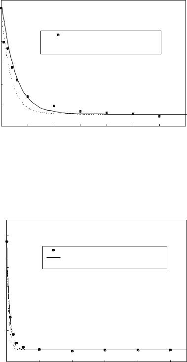
Figures 2 to 4 show experimental data for ion flotation of cupric ion by SDS, STS, and SHS, along with the curves predicted by equations 3 and 4. It is evident that the predictions with a constant bubble diameter overestimated the metal removal rate, especially at longer flotation times. After correcting for the bubble diameter, using equation 4, the predicted copper concentrations agreed well with the experimental data for most of the duration of the ion flotation tests.
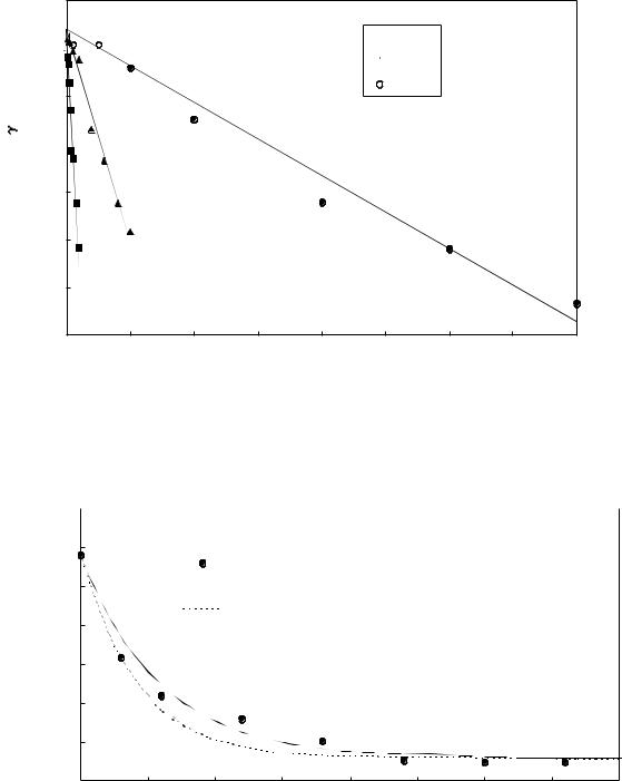
Surface tension (N/m)
0.075

 SHS-Cu 0.07


 STS-Cu
 SDS-Cu
0.065
0.06 
0.055
0.05
0.045
0.04
0 0.0001 0.0002 0.0003 0.0004 0.0005 0.0006 0.0007 0.0008
Surfactant concentrationC A - (M
Figure 1: Surface tensions of SDS-Cu, STS-Cu and SHS-Cu solutions as a function of alkylsulfate concentration. Copper and alkylsulfate were present in stoichiometric ratios. Ionic strength was 3 mM for SDS-Cu, and 1 mM for STS-Cu and SHS-Cu.
[Cu] (M)
0.00035 |
|
|
|
|
|
|
|
|
|
|
|
0.0003 |
|
|
|
|
|
|
|
|
|
SDS-Cu (experimental) |
|
0.00025 |
|
|
|
SDS-Cu (predicted, with bubble diameter correction) |
|
|
|
|
|
||
|
|
|
|
SDS-Cu (predicted, constant bubble diameter) |
|
0.0002 |
|
|
|
|
|
|
|
|
|
|
0.00015
0.0001
0.00005
0
0 |
50 |
100 |
150 |
200 |
250 |
300 |
350 |
400 |
Time(min)
Figure 2: Copper ion removal in the SDS-Cu ion flotation system. Air flow rate Qair = 20 ml/min, solution charge V=650 ml. Initial copper and SDS concentrations are 0.29 mmol/Land 0.58 mmol./L respectively. Broken line predicted from equation 3, assuming constant bubble diameter db,0=8x10⁻⁵m. Solid line predicted from equation 4, with surface tension-dependent bubble diameter
[Cu] (M)
0.00003
0.000025
STS-Cu (experimental)
0.00002 |
|
STS-Cu (predicted, with bubble diameter correction) |
|


 STS-Cu(predicted, constant bubble diameter)
0.000015
0.00001
0.000005
0
0 |
20 |
40 |
60 |
80 |
100 |
120 |
140 |
Time (min)
Figure 3: Copper ion removal in the STS-Cu ion flotation system. Air flow rate Qair = 20 ml/min, solution charge V=650 ml. Initial copper and STS concentrations are 28.1 mol/Land 56.2 mol./L respectively. Broken line predicted from equation 3, assuming constant bubble diameter db,0=8x10⁻⁵m. Solid line predicted from equation 4, using surface tension-dependent bubble diameter, with db,0=9.55x10⁻⁵m.
0.000008
|
0.000006 |
[Cu] (M) |
0.000004 |
0.000002
0
0
SHS-Cu (experimental)
SHS-Cu (predicted, with bubble diameter correction) 


 SHS-Cu (predicted, constant bubble diameter)
20 |
40 |
60 |
80 |
100 |
|
|
Time (min) |
|
|
Figure 4: Copper ion removal in the SHS-Cu ion flotation system. Air flow rate Qair = 20 ml/min, solution charge V=650 ml. Initial copper and SHS concentrations are 7.64 mol/L and 15.3 mol/L respectively. Broken line predicted from equation 3, assuming constant bubble diameter db,0=8x10⁻⁵m. Solid line predicted from equation 4, using surface tension-dependent bubble diameter, with db,0=8.512x10⁻⁵m..

Table 1: Physicochemical parameters and their
effects on ion flotation performance
|
|
|
Effects on |
|
|
||
Parameters |
|
metal removal |
Examples |
||||
|
|
|
rate |
RM n+ |
|
|
|
|
Air flow |
rate |
RM n+ |
↑ as |
Sreenivasarao, |
||
|
(Qair) |
|
Qair ↑ |
|
1996 |
|
|
|
|
|
|
|
|
||
|
Average |
|
RM n+ ↑ as db ↓ |
Pinfold, 1972 |
|||
Physical |
bubble |
|
|
|
|
|
|
diameter (db) |
|
|
|
|
|
||
Parameters |
|
|
|
|
|
||
|
Solution |
|
RM n+ ↑ as |
V |
Sreenivasarao, |
||
|
Volume(V) |
↓ |
|
1996 |
|
||
|
|
|
|
|
|
||
|
Temperature |
RM n+ ↑ as |
T ↓ |
Morgan, 1992 |
|||
|
(T) |
|
|
|
|
Pinfold, 1972 |
|
|
Initial |
|
RM n+ ↑ as |
C0 |
Valdes-Krieg, |
||
|
colligend |
|
↑ |
|
1977 |
|
|
|
concentration |
|
|
|
|||
|
|
|
|
|
|
||
|
(C0) |
|
|
|
|
|
|
|
Surface |
|
RM n+ ↑ as |
b ↑ |
Doyle |
and Liu, |
|
|
activity of |
|
|
|
|
1999, |
|
Chemical |
collector and |
|
|
|
Sreenivasarao, |
||
parameters |
colligend (b) |
|
|
|
1996 |
|
|
|
Charge |
on |
RM n+ ↑ as n ↑ |
Duyvesteyn, |
|||
|
colligend |
|
(pH and ionic |
1994, |
Pinfold |
||
|
(n) |
|
1972 |
|
|||
|
|
strength can |
|
||||
|
|
|
|
|
|||
|
|
|
modify n) |
|
|
|
|
|
Power |
of |
As power of |
Duyvesteyn, |
|||
|
frother |
|
frother↑ |
|
1994, |
Pinfold |
|
|
|
|
backflux |
|
1972 |
|
|
|
|
|
decreases, |
|
|
||
|
|
|
hence |
RM n+ ↑ |
|
|
|
Equations 3 and 4 incorporate various physicochemical parameters that are adjustable during ion flotation. Table 1 summarizes these different parameters and indicates how altering them should affect the metal ion removal rate. A few references that are consistent with these predictions are cited.
Modeling Metal Ion Selectivity Coefficients
A model was developed to calculate the selectivity coefficient for two competing metal ions with the same charge at the solution-vapor interface. This model geometrically calculates α, the fraction of the complete secondary hydration sphere that becomes dehydrated when the metal ion approaches the vapor/solution interface:
α = |
1 |
− |
(rion + 2rw + rs )2 − rs 2 |
(5) |
|
2 |
2(r + 2r + r ) |
|
|||
|
|
|
ion |
w s |
|
where rion, rw, and rs are the crystal ionic radius of the metal ion, the radius of the water molecule, and the radius of the
functional group on the surfactant, respectively.
This is used to estimate the portion of the Gibbs free energy for adsorption due to dehydration, Godehydr:
Table 2: Data for calculating Godehydr
Met |
rion(10-10m) |
δ |
Gosec |
α |
Godehydr |
al |
(Dean, |
(10-10m) |
dehydr |
|
(J/mole) |
ion |
1978) |
|
(J/mole) |
|
|
Cu2+ |
0.72 |
9.04 |
122651.1 |
0.050243 |
6162.396 |
Ca2+ |
0.99 |
9.61 |
113820.2 |
0.045916 |
5226.136 |
Pb2+ |
1.20 |
10.05 |
107784.3 |
0.042931 |
4627.341 |
rw=1.38x10⁻¹⁰m (James and Healy 1972), |
rs(SDS)=2.7x10⁻¹⁰m |
||||
Table 3: Comparison of experimental selectivity coefficients with those predicted by dehydration and surface tension models
|
Experimental |
Dehydration |
Surface |
|
measurement |
Model |
tension |
|
|
|
model |
|
|
|
|
βCa2 + / Cu2 + |
1.438 |
1.551 |
1.115 |
|
|
|
|
βPb2 + / Cu2 + |
2.138 |
2.066 |
1.686 |
|
|
|
|
G0dehydr = αΔG0sec dehydr = |
αn2e2N |
|
|
( |
1 |
− |
1 |
) (6) |
|
8π( r |
+ 2r |
)ε |
0 |
6 |
78.5 |
||||
|
ion |
w |
|
|
|
|
|
|
|
Incorporation into the Grahame adsorption equation then yields (Liu and Doyle, 1999):
|
|
|
|
|
( |
α2 |
− |
α1 |
) |
n2e2 N |
( |
1 |
− |
1 |
) |
|
|
|
|
|
|
n+ = |
|
|
|
|
|
|
(7) |
||||||||
β |
n+ |
/ M2 |
δ1 |
exp[ |
|
rion2 +2rw |
|
rion1 +2rw |
|
8πε0 |
6 |
|
78.5 |
|
] |
|||
|
|
|
|
|
|
|
|
|
|
|
|
|||||||
|
M1 |
|
δ2 |
|
|
|
|
RT |
|
|
|
|
|
|
|
|
|
|
|
|
|
|
|
|
|
|
|
|
|
|
|
|
|
|
|
||
where |
βM1n+ / M2n+ is the selectivity coefficient between two metal |
|||||||||||||||||
ions with charge n+. δ is the thickness of the surface layer into which the metal ions are adsorbed. N is the Avogadro number, ε0 is the permeability of a vacuum, and 78.5 is the dielectric constant of water in the bulk solution at 25°C. The dielectric constant of water in a very high electric field at the vapor/solution interface is taken to be 6. The subscripts 1 and 2 denote the two different metal ions.
Table 2 lists the parameters identified above, including the
theoretically calculated α and dehydration energy ( Godehydr). It is evident that the larger the ionic crystal radius, the lower are
α and Godehydr. Hence, from equation 7, the higher will be the selectivity for this metal ion.
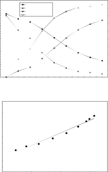
Figures 5 and 6 show the concentrations and removals of Cu2+, Ca2+ and P b2+ during ion flotation from mixed-metal solutions using dodecylsulfate. Following the method of Morgan et al. (1994), the selectivity coefficients were
determined from the gradient of plots of lnCM2+ versus lnCCu2+ (also shown in Figures 5 and 6). The experimental and
theoretical selectivity coefficients, βM1n+ / M2n+ , are shown in Table
3. It is evident that the selectivity coefficients predicted by the dehydration model agree well with the experimentally measured selectivity coefficients.
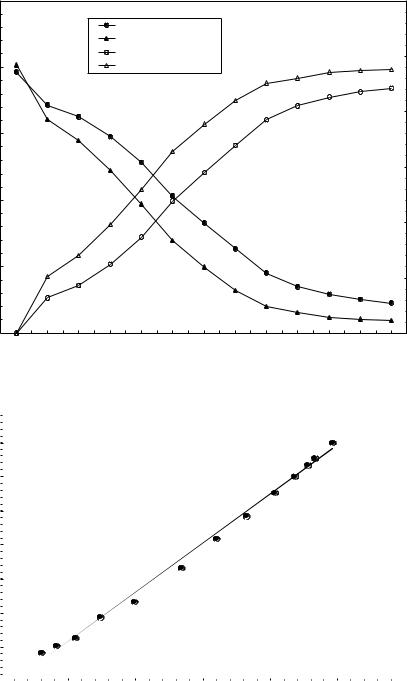
0.00025 |
|
|
|
|
|
|
|
|
|
|
|
120 |
|
|
|
|
|
[Cu](M) |
|
|
|
|
|
|
|
|
|
|
|
|
|
[Ca](M) |
|
|
|
|
|
|
|
|
|
|
|
|
|
Percent removal of Cu (%) |
|
|
|
|
|
100 |
|
||
|
|
|
|
Percent removal of Ca(%) |
|
|
|
|
|
|
|||
0.0002 |
|
|
|
|
|
|
|
|
|
|
|||
|
|
|
|
|
|
|
|
|
|
|
|
|
|
|
|
|
|
|
|
|
|
|
|
|
|
80 |
of metal ions (%) |
0.00015 |
|
|
|
|
|
|
|
|
|
|
|
|
|
concentration(M) |
|
|
|
|
|
|
|
|
|
|
|
60 |
|
|
|
|
|
|
|
|
|
|
|
|
|
|
|
0.0001 |
|
|
|
|
|
|
|
|
|
|
|
|
|
Residue metalion |
|
|
|
|
|
|
|
|
|
|
|
40 |
Percentremoval |
|
|
|
|
|
|
|
|
|
|
|
|
||
0.00005 |
|
|
|
|
|
|
|
|
|
|
|
|
|
|
|
|
|
|
|
|
|
|
|
|
|
20 |
|
0 |
|
|
|
|
|
|
|
|
|
|
|
0 |
|
0 |
20 |
40 |
60 |
90 |
120 |
150 |
180 |
210 |
240 |
270 |
300 |
330 |
|
Time (minutes)
Ln[Ca]
-8 |
|
|
|
|
|
|
|
|
|
|
|
|
|
|
|
|
|
|
|
|
|
|
|
|
|
|
|
|
|
-8.5 |
|
|
|
|
|
|
|
|
|
|
y = 1.4379x + 3.6697 |
|
|
|
|
|
|
|
|
|
|
|
|
|
|||||
|
|
|
|
|
|
|
|
|
|
|
|
|
|
|
|
|
|
|
|
|
|
|
|||||||
|
|
|
|
|
|
|
|
|
|
|
|
|
|
|
|
|
|
|
|
|
|
|
|
||||||
|
|
|
|
|
|
|
|
|
|
|
|
|
|
|
|
|
|
|
|
|
|||||||||
-9 |
|
|
|
|
|
|
|
|
|
|
R2 |
= 0.9955 |
|
|
|
|
|
|
|
|
|
|
|
|
|
|
|||
|
|
|
|
|
|
|
|
|
|
|
|
|
|
|
|
|
|
|
|
|
|
|
|
||||||
|
|
|
|
|
|
|
|
|
|
|
|
|
|
|
|
|
|
|
|
||||||||||
|
|
|
|
|
|
|
|
|
|
|
|
|
|
|
|
|
|
|
|
|
|
|
|
|
|
|
|
|
|
-9.5 |
|
|
|
|
|
|
|
|
|
|
|
|
|
|
|
|
|
|
|
|
|
|
|
|
|
|
|
|
|
|
|
|
|
|
|
|
|
|
|
|
|
|
|
|
|
|
|
|
|
|
|
|
|
|
|
|
|
|
|
|
|
|
|
|
|
|
|
|
|
|
|
|
|
|
|
|
|
|
|
|
|
|
|
|
|
|
|
|
|
-10 |
|
|
|
|
|
|
|
|
|
|
|
|
|
|
|
|
|
|
|
|
|
|
|
|
|
|
|
|
|
|
|
|
|
|
|
|
|
|
|
|
|
|
|
|
|
|
|
|
|
|
|
|
|
|
|
|
|
|
|
|
|
|
|
|
|
|
|
|
|
|
|
|
|
|
|
|
|
|
|
|
|
|
|
|
|
|
|
|
|
|
|
|
|
|
|
|
|
|
|
|
|
|
|
|
|
|
|
|
|
|
|
|
|
|
|
|
|
|
|
-10.5 |
|
|
|
|
|
|
|
|
|
|
|
|
|
|
|
|
|
|
|
|
|
|
|
|
|
|
|
|
|
|
|
|
|
|
|
|
|
|
|
|
|
|
|
|
|
|
|
|
|
|
|
|
|
|
|
|
|
|
|
|
|
|
|
|
|
|
|
|
|
|
|
|
|
|
|
|
|
|
|
|
|
|
|
|
|
|
|
|
|
-11 |
|
|
|
|
|
|
|
|
|
|
|
|
|
|
|
|
|
|
|
|
|
|
|
|
|
|
|
|
|
|
|
|
|
|
|
|
|
|
|
|
|
|
|
|
|
|
|
|
|
|
|
|
|
|
|
|
|
|
|
|
|
|
|
|
|
|
|
|
|
|
|
|
|
|
|
|
|
|
|
|
|
|
|
|
|
|
|
|
|
|
|
|
|
|
|
|
|
|
|
|
|
|
|
|
|
|
|
|
|
|
|
|
|
|
|
|
|
|
|
-11.5 |
|
|
|
|
|
|
|
|
|
|
|
|
|
|
|
|
|
|
|
|
|
|
|
|
|
|
|
|
|
|
|
|
|
|
|
|
|
|
|
|
|
|
|
|
|
|
|
|
|
|
|
|
|
|
|
|
|
|
|
|
|
|
|
|
|
|
|
|
|
|
|
|
|
|
|
|
|
|
|
|
|
|
|
|
|
|
|
|
|
|
|
|
|
|
|
|
|
|
|
|
|
|
|
|
|
|
|
|
|
|
|
|
|
|
|
|
|
|
|
|
|
|
|
|
|
|
|
|
|
|
|
|
|
|
|
|
|
|
|
|
|
|
|
|
|
|
|
|
|
|
|
|
|
|
|
|
|
|
|
|
|
|
|
|
|
|
|
|
|
|
|
|
|
|
|
|
|
|
|
-12 |
|
|
|
|
|
|
|
|
|
|
|
|
|
|
|
|
|
|
|
|
|
|
|
|
|
|
|
|
|
|
|
|
|
|
|
|
|
|
|
|
|
|
|
|
|
|
|
|
|
|
|
|
|
|
|
|
|
|
|
|
|
|
|
|
|
|
|
|
|
|
|
|
|
|
|
|
|
|
|
|
|
|
|
|
|
|
|
|
|
-11 |
|
|
-10.5 |
-10 |
-9.5 |
|
|
|
-9 |
|
|
|
|
|
-8.5 |
-8 |
|||||||||||||
Ln[Cu]
Figure 5: Selective ion flotation in SDS-Cu2+-Ca2+ system. Initial feed solution composition: [SDS] = 0.8mM, [Cu2+]=[Ca2+] = 0.2mM, ethanol = 0.4% (v/v), pH = 3.80. Airflow rate Qair: 20ml/min, solution charge, V= 650 ml.
0.00012 |
|
|
|
|
|
|
|
100 |
|
|
|
[Cu](M) |
|
|
|
|
|
|
|
|
|
[Pb](M) |
|
|
|
|
|
90 |
|
0.0001 |
|
Percent removal of Cu(%) |
|
|
|
|
|
|
|
|
Percent removal of Pb(%) |
|
|
|
|
|
|
||
|
|
|
|
|
|
80 |
|
||
|
|
|
|
|
|
|
|
|
|
|
|
|
|
|
|
|
|
70 |
|
0.00008 |
|
|
|
|
|
|
|
|
|
concentration(M) |
|
|
|
|
|
|
|
60 |
ofmetalions(%) |
|
|
|
|
|
|
|
50 |
||
0.00006 |
|
|
|
|
|
|
|
|
|
|
|
|
|
|
|
|
|
40 |
|
0.00004 |
|
|
|
|
|
|
|
|
|
Residuemetalion |
|
|
|
|
|
|
|
30 |
removalPercent |
|
|
|
|
|
|
|
|
||
|
|
|
|
|
|
|
|
20 |
|
0.00002 |
|
|
|
|
|
|
|
|
|
|
|
|
|
|
|
|
|
10 |
|
0 |
|
|
|
|
|
|
|
0 |
|
0 |
10 |
20 |
40 |
60 |
80 |
100 |
120 |
150 |
|
Time (minutes)
|
-8 |
|
|
|
|
-9 |
|
y = 2.1378x + 10.264 |
|
|
|
|
|
|
|
|
|
R2 = 0.976 |
|
|
-10 |
|
|
|
Ln[Pb] |
-11 |
|
|
|
|
|
|
|
|
|
-12 |
|
|
|
|
-13 |
|
|
|
|
-14 |
|
|
|
|
-10.8 |
-10.3 |
-9.8 |
-9.3 |
|
|
|
Ln[Cu] |
|
Figure 6: Selective ion flotation in SDS-Cu2+-Pb2+ system. Initial feed solution composition: [SDS] = 0.4mM, [Cu2+]=[Pb2+] = 0.1mM, ethanol = 0.4% (v/v), pH = 4.02. Airflow rate, Qair: 20ml/min, solution charge = 650 ml.
Table 4: Surface tensions of solutions in the SDSCu, SDS-Ca and SDS-Pb systems
System |
γ = γo – bCDS-, mN/m |
R2 |
|
SDS-Cu2+ |
γ = 70.031 |
– 42049CDS- |
0.9718 |
SDS-Ca2+ |
γ = 69.203 |
– 46900CDS- |
0.9779 |
SDS-Pb2+ |
γ = 69.674 |
- 70904CDS- |
0.9905 |
We have also defined a pseudo-selectivity coefficient β 'M1n+ / M2n+ based on surface tension data (Liu and Doyle,
1999). Figure 1 showed that the surface tension, γ, of a solution of SDS and Cu2+, present in stoichiometric ratio, is given by:
γ = γo – bCDS- |
(8) |
|||
The pseudo-selectivity coefficient is defined as: |
|
|||
β 'M1n+ / M2n+ = |
b1 |
|
(9) |
|
b |
||||
|
|
|||
2 |
|
|
||
where b1 and b2 are the negative gradients of plots similar to Figure 1, for different metal ions. Table 4 gives the experimentally determined equations of these curves for the SDS-Cu, SDS-Ca and SDS-Pb systems. It is evident from the high R2 values that the surface tension data did, indeed, follow the linear relationship of equation 8. Table 3 shows the pseudo-selectivity coefficients determined from the gradients appearing in Table 4, using equation 9. It is clear that the surface tension model gives a rather poor prediction of the selectivity coefficient, although it does predict the correct order of selectivity. The probable reason for the poor predictions of the surface tension model is that this model takes data from single-colligend systems, and uses these to predict the behavior in mixed colligend systems, ignoring any interactions.
CONCLUSIONS
Surface tension data have been successfully used to quantitatively predict the rates of metal ion removal during ion flotation with alkylsulfates. The selectivity for the metal ions C u2+, Ca2+ and Pb2+ during ion flotation with dodecylsulfate agreed very well with a thermodynamic model that considered the amount of dehydration that accompanies adsorption of the metal ion at the vaporsolution interface. A model for selectivities based on surface tension measurements gives a rather poor prediction of metal ion selectivity coefficients, although it did qualitatively predict the correct order of the selectivity sequence.
REFERENCES
Clarke, A. N. and Wilson, D. J., 1983, Foam Flotation: Theory and Applications, Marcel Dekker, New York.
Dean, J. A., 1978, Lange’s Handbook of Chemistry, 12th edition, McGraw-Hill Inc.
Doyle F. M., Duyvesteyn, S. and Sreenivasarao, K., 1995, “The use of ion flotation for detoxification of metalcontaminated waters and process effluents” Proceedings of XIX International Mineral Processing Congress, Vol.4, SME, Littleton, CO, pp. 175-179.
Doyle, F. M. and Liu, Z., 1999, “A thermodynamic approach to ion flotation. I. Kinetics of cupric ion flotation with alkylsulfates”, submitted to Colloids and Surfaces.
Duyvesteyn, S., 1994, “Removal of Trace Metal Ions from Dilute Solutions by Ion Flotation: Cadium-Dodecylsulfate and Copper-Dodecylsulfate Systems”, Master Thesis, University of California, Berkeley.
Grieves, R. B. and Kyle, R. N., 1982, “Models for interactions between ionic surfactants and nonsurfaceactive ions in foam fractionation processes”, Separation Science and Technology, Vol. 17(3), pp. 465-483.
Grieves, R. B., Burton, K.E. and Craigmyle, J. A., 1987, “Experimental foam fractionation selectivity coefficients for the alkali (Group IA) metals”, Separation Science and Technology, Vol. 22 (6), pp. 1597-1608.
Huang, R.C.H., and Talbot, F.D., 1973, “The removal of copper, cadmium and lead ions from dilute aqueous solutions using foam fractionation”, Canadian Journal of Chemical Engineering, Vol. 51, pp. 709-713.
Huang, S., Ho, H., Li, Y. and Lin, C., 1995, “Adsorbing colloid flotation of heavy metal ions from aqueous solutions at large ionic strength”, Environmental Science and Technology, Vol. 29, pp. 1802-1807.
James, R. O. and Healy, T. W., 1972, “Adsorption of hydrolyzable metal ions at the oxide-water interface III. A thermodynamic model of adsorption”, Journal of Colloid and Interface Science, Vol.40, No.1, July pp. 65-81.
Jorne, J. and Rubin, E., 1969, “Ion fractionation by foam”, Separation Science, Vol. 4 (4), August, pp.313-324.
Liu, Z. and Doyle, F. M., 1999, “A thermodynamic approach to ion flotation. II. metal ion selectivity in the SDS- Cu-Ca and SDS-Cu-Pb Systems”, Submitted to Colloids and Surfaces.
Morgan, J. D., Napper, D. H., Warr, G. G., Nicol, S. K., 1992, “Kinetics of recovery of hexadecyltrimethylammonium bromide by flotation”, Langmuir, Vol. 8, pp. 2124-2129.
Morgan, J. D., Napper, D. H., Warr, G. G. and Nicol, S. K., 1994, “Measurement of the selective adsorption of ions at air/surfactant solution interfaces”, Langmuir, Vol. 10, pp. 797-801.
Morgan, J. D., Napper, D. H. and Warr, G. G., 1995, "Thermodynamics of ion exchange selectivity", Journal of Physical Chemistry, Vol. 99, pp. 9458-9465.
Okamoto, Y., Chou, E.J., 1976, “Chelation Effects of Surfactant in Foam Separation: Removal of Cadmium and Copper Ions from Aqueous Solution”, Separation Science, Vol. 11 (1), pp. 79-87.
Pinfold, T. A., 1972, “Ion flotation”, Adsorptive Bubble Separation Techniques, Edited by R. Lemlich, Academic Press.
Sebba, F., 1959, Nature, Vol. 184, p. 1062.
Sreenivasarao, K., 1996, “Removal of toxic metals from dilute synthetic solutions by ion and precipitate flotation”, Ph.D dissertation, University of California, Berkeley.
Sreenivasarao, K., Doyle, F. M. and Fuerstenau, D. W., 1993, “Removal of toxic metals from dilute effluents by ion flotation”, EPD Congress’93, Edited by J.P.Hager, TMS, Warrendale, PA, pp.45-56.
Valdes-Krieg, E. et al., 1977, “Separation of cations by foam and bubble fractionation”, Separation and Purification Methods, Vol. 6 (2), pp. 221-285.
Walkowiak, W., 1991, “Mechanism of selective ion flotation. 1. Selective flotation of transitional metal cations”, Separation Science and Technology, Vol. 26 (4), pp.559-568.