Encyclopedia of SociologyVol._1

other locales. In addition, the very size of many multinationals restricts the pressure that either the home or the host country can impose.

Through various actions corporations demonstrate that they are attentive to the societies they inhabit. Corporate leaders serve on the boards of social service agencies; corporate foundations provide funds for community programs; employees donate their time to local causes. The agenda of corporations long have included these and similar activities. Increasingly, the agenda organize such actions around the idea of corporate social responsibility. Acting responsibly means taking steps to promote the commonweal (Steckmest 1982).

Some corporations strive more consistently to advance social ends than do others. Differences in norms and values apparently explain the contrast. Norms, or maxims for behavior, indicate the culture of the organization (Deal and Kennedy 1982). The culture of some settings gives the highest priority to actions that protect the health, safety, and welfare of citizens and their heirs. Elsewhere, those are not what the culture emphasizes (Clinard 1983; Victor and Cullen 1988).

The large corporation had become such a dominant force by the 1980s that no one envisioned a return to an era of small, diffuse organizations. Yet, during that decade some sectors had started to move from growth to contraction. At times, the shift resulted from legislative action. When the Bell Telephone System divided in 1984, by order of the courts, the change marked a sharp reversal. For more than a century the system had glided toward integration and standardization (Barnett and Carroll 1987; Barnett 1990).

Whether through fiat or choice, corporations contract (Whetten 1987; Hambrick and D’Aveni 1988). Two perspectives associate the rise and fall in the fortunes of corporations to changes in the social context. The first perspective, resource dependence, centers on the idea that organizations must secure their resources from their environs (McCarthy and Zald 1977; Jenkins 1983). When those environs contain a wealth of resources— personnel in the numbers and with the qualifications the organization requires, funds to finance operations—the corporation can thrive. When hard times plague the environs, the corporation escapes that fate only with great difficulty.

The perspective known as population ecology likewise connects the destiny of organizations to conditions in their surroundings. Population ecologists think of organizations as members of a population. Changing social conditions can enrich or impoverish a population. Individual units within it can do little to offset the tide of events that threatens to envelop the entire population. (Hannan and Freeman 1988; Wholey and Brittain 1989; for a critique of the approach see Young 1988).

Neither resource dependency theory nor population ecology theory focuses explicity on the corporate form. But just as analyses of corporations inform the discussions sociologists have undertaken on formal organizations, models drawn from studies of organizations have proved useful as scholars have tracked the progress of corporations.

The corporation clearly constitutes a power to be reckoned with. As with its precursors, the modern corporation serves needs that collectivities develop. In fact, the corporation rests on an assumption that is fundamental in sociology: A collectivity has an identity of its own. But the corporation of the twentieth century touches more than those persons who own its assets or produce its goods. This social instrument of the Middle Ages is now a social fixture.

(SEE ALSO: Capitalism; Organizational Effectiveness;

Organizational Structure; Transnational Corporations)

REFERENCES

Antai, Ariane-Berthoin 1992 Corporate Social Performance: Rediscovering Actors in Their Organizational Contexts. Boulder, Colo.: Westview Press.

Barnett, William P. 1990 ‘‘The Organizational Ecology of a Technological System.’’ Administrative Science Quarterly 35:31–60.

Barnett, William P., and Glenn Carroll 1987 ‘‘Competition and Mutualism Among Early Telephone Companies.’’ Administrative Science Quarterly 32:400–421.

Berg, Ivar, and Mayer N. Zald 1978 ‘‘Business and Society.’’ Annual Review of Sociology 4:115–143.

Berle, Adolph A., and Gardiner C. Means 1932 The

Modern Corporation and Private Property. New York:

Macmillan.

Braverman, Harry 1974 Labor and Monopoly Capital: The Degradation of Work in the Twentieth Century. New York: Monthly Review.

Breedlove, William L., and J. Michael Armer 1996 ‘‘Economic Disarticulation and Social Development in Less-Developed Nations: A Cross-National Study of Intervening Structures.’’ Sociological Focus 29:359–378.

Burawoy, Michael 1979 Manufacturing Consent: Changes in the Labor Process under Monopoly Capitalism. Chicago: University of Chicago Press.

———1985 The Politics of Production: Factory Regimes under Capitalism and Socialism. London: Verso.

Chandler, Alfred D., Jr. 1962 Strategy and Structure. Cambridge, Mass.: MIT Press.

———1977 The Visible Hand. Cambridge, Mass.: Har-

vard University Press.

———1980 ‘‘The United States: Seedbed of Managerial Capitalism.’’ In A. D. Chandler, Jr., and Herman Daems, eds., Managerial Hierarchies. Cambridge, Mass.: Harvard University Press.

———1984 ‘‘The Emergence of Managerial Capitalism.’’ Business History Review 58:484–504.

Clawson, Dan 1980 Bureaucracy and the Labor Process. New York: Monthly Labor Review.

Clinard, Marshall B. 1983 Corporate Ethics and Crime. Beverly Hills, Calif.: Sage.

———, and Peter C. Yeager 1980 Corporate Crime. New York: Free Press.

Coleman, James S. 1974 Power and the Structure of Society. New York: Norton.

Coleman, James S. 1996 ‘‘The Asymmetric Society: Organizational Actors, Corporate Power, and the Irrelevance of Persons.’’ In M. David Ermann, and Richard J.Lundman, eds., Corporate and Governmental Deviance: Problems of Organizational Behavior in Contemporary Society. New York: Oxford University Press.

Cuthbert, Alexander R., and Keith G. McKinnell 1997 ‘‘Ambiguous Space, Ambiguous Rights-Corporate Power and Social Control in Hong Kong.’’ Cities 14: 295–311.

Davis, Gerald F. 1994 ‘‘The Corporate Elite and the Politics of Corporate Control.’’ Current Perspectives in Social Theory 1: 215–238.

Davis, Gerald F., Kristina A. Diekmann, and Catherine H. Tinsley. 1994. ‘‘The Decline and Fall of the Conglomerate Firm in the 1980s: The Deinstitutionalization of an Organizational Form.’’ American Sociological Review 59: 547–570.

Deal, Terrence, and Allen Kennedy 1982 Corporate Culture. Reading, Mass.: Addison-Wesley.

DiMaggio, Paul 1988 ‘‘Interest and Agency in Institutional Theory.’’ In Lynne G. Zucker, ed., Research on

Institutional Patterns: Environment and Culture. Cambridge, Mass.: Ballinger.

———, and Walter Powell 1983 ‘‘The Iron Cage Revisited: Institutional Isomorphism and Collective Rationality in Organizational Fields.’’ American Sociological Review 48:147–160.

Donaldson, Thomas 1992 ‘‘Individual Rights and Multinational Corporate Responsibilities.’’ National Forum 72: 7–9.

Dunford, Louise, and Ann Ridley 1996 ‘‘No Soul to Be Damned, No Body to Be Kicked: Responsibility, Blame and Corporate Punishment.’’ International Journal of the Sociology of Law 24:1–19.

Dunworth, Terence, and Joel Rogers 1996 ‘‘Corporations in Court: Big Business Litigation in U.S. Federal Courts, 1971–1991.’’ Law and Social Inquiry 21: 497–592.

Edwards, Richard 1979 Contested Terrain: The Transformation of the Workplace in the Twentieth Century. New York: Basic Books.

Etzioni, Amitai 1993 ‘‘The U.S. Sentencing Commission on Corporate Crime: A Critique.’’ Annals of the American Academy of Political and Social Science 525: 147–156.

Hambrick, Donald C., and Richard A. D’Aveni 1988 ‘‘Large Corporate Failures as Downward Spirals.’’

Administrative Science Quarterly 33:1–23.

Hannan, Michael, and John Freeman 1988 Organizational Ecology. Cambridge, Mass.: Harvard University Press.

Hawley, James P. 1995 ‘‘Political Voice, Fiduciary Activism, and the Institutional Ownership of U.S. Corporations: The Role of Public and Noncorporate Pension Funds.’’ Sociological Perspectives 38:415–435.

Ireland, Paddy 1996 ‘‘Corporate Governance, Stakeholding, and the Company: Towards a Less Degenerate Capitalism?’’ Journal of Law and Society 23:287–320.

Jacoby, Sanford 1985 Employing Bureaucracy: Managers, Unions and the Transformation of Work in American Industry, 1900–1945. New York: Columbia University Press.

Jenkins, J. Craig 1983 ‘‘Resource Mobilization Theory and the Study of Social Movements.’’ Annual Review of Sociology 42:249–268.

Jones, Marc T. 1996 ‘‘The Poverty of Corporate Social Responsibility.’’ Quarterly Journal of Ideology 19:1–2.

Lofquist, William S. 1993 ‘‘Legislating Organizational Probation: State Capacity, Business Power, and Corporate Crime Control.’’ Law and Society Review 27: 741–783.

Luchansky, Bill, and Gregory Hooks 1996 ‘‘Corporate Beneficiaries of the Mid-Century Wars: Respecifying

Models of Corporate Growth, 1939–1959.’’ Social

Science Quarterly 77:301–313.

McCarthy, John D., and Mayer N. Zald 1977 ‘‘Resource Mobilization and Social Movements: A Partial Theory.’’ American Journal of Sociology 82:1212–1241.

McKinlay, Alan, and Ken Starkey 1998 Foucalt, Management and Organizations Theory: From Panopticion to Technologies of Self. London: Sage Publications.

Mechanic, David 1962 ‘‘Sources of Power of Lower Participants in Complex Organizations.’’Administrative Science Quarterly 7:349–364.

Meyer, John, and Brian Rowan 1977 ‘‘Institutionalized Organizations: Formal Structure as Myth and Ceremony.’’ American Sociological Review 83:340–363.

Mintz, Beth, and Michael Schwartz 1985 The Power Structure of American Business. Chicago: University of Chicago Press.

Nelson, Daniel 1975 Managers and Workers. Madison: University of Wisconsin Press.

Parker-Gwin, Rachel, and William G. Roy 1996 ‘‘Corporate Law and the Organization of Property in the United States: The Origin and Institutionalization of New Jersey Corporation Law, 1888–1903.’’ Politics and Society 24:111–135.

Prechel, Harland 1994 ‘‘Economic Crisis and the Centralization of Control over the Managerial Process: Corporate Restructuring and Neo-Fordist DecisionMaking.’’ American Sociological Review 59:723–745.

Ridley, Ann, and Louise Dunford 1994 ‘‘Corporate Liability for Manslaughter: Reform and the Art of the Possible.’’ International Journal of the Sociology of Law 22:309–328.

Rodman, Kenneth A. 1995 ‘‘Sanctions at Bay? Hegemonic Decline, Multinational Corporations, and U.S. Economic Sanctions since the Pipeline Case.’’ International Organization 49:105–137.

Roy, Donald 1952 ‘‘Restriction of Output in a Piecework Machine Shop.’’ Ph.D. diss., University of Chicago, Chicago.

Sutherland, Edwin H. 1949 White Collar Crime. New York: Holt, Rinehart, and Winston.

Tolbert, Pamela S., and Lynne G. Zucker 1983 ‘‘Institutional Sources of Change in the Formal Structure of Organizations: The Diffusion of Civil Service Reform, 1880–1935.’’ Administrative Science Quarterly

28:22–39.

Useem, Michael 1984 The Inner Circle: Large Corporations and the Rise of Political Activity in the U.S. and U.K. New York: Oxford University Press.

Victor, Bart, and John B. Cullen 1988 ‘‘The Organizational Bases of Ethical Work Climates.’’ Administrative Science Quarterly 33:101–125.

Westphal, James D., and Edward J. Zajac 1997 ‘‘Defections from the Inner Circle: Social Exchange, Reciprocity, and the Diffusion of Board Independence in U.S. Corporations.’’ Administrative Science Quarterly

42:161–183.

Whetten, David A. 1987 ‘‘Organizational Growth and Decline Processes.’’ Annual Review of Sociology

13:335–358.

Wholey, Douglas, and Jack Brittain 1989 ‘‘Characterizing Environmental Variation.’’ Academy of Management Journal 32:867–882.

Wilks, Stephen 1992 ‘‘Science, Technology and the Large Corporation.’’ Government and Opposition

27:190–212.

Young, Ruth 1988 ‘‘Is Population Ecology a Useful Paradigm for the Study of Organizations?’’ American Journal of Sociology 94:1–24.

Zeitlin, Maurice 1974 ‘‘Corporate Ownership and Control: The Large Corporation and the Capitalist Class.’’

American Journal of Sociology 79:1073–1119.

Zey, Mary, and Brande Camp 1996 ‘‘The Transformation from Multidimensional Form to Corporate Groups of Subsidies in the 1980s: Capital Crisis Theory.’’ Sociological Quarterly 37:327–351.

CORA B. MARRETT

Sanders, Joseph, and V. Lee Hamilton 1996 ‘‘Distributing Responsibility for Wrongdoing inside Corporate Hierarchies: Public Judgments in Three Societies.’’

Law and Social Inquiry 21:815–855.

Scott, W. Richard 1987 ‘‘The Adolescence of Institutional Theory.’’ Administrative Science Quarterly

32:493–511.

Steckmest, Francis W. 1982 Corporate Performance: The Key to Public Trust. New York: McGraw-Hill.

Stone, Christopher D. 1975 Where the Law Ends: The Social Control of Corporate Behavior. New York: Harper.

CORRECTIONS SYSTEMS

See Penology; Criminal Sanctions; Criminology.

CORRELATION AND REGRESSION ANALYSIS

In 1885, Francis Galton, a British biologist, published a paper in which he demonstrated with graphs and tables that the children of very tall

parents were, on average, shorter than their parents, while the children of very short parents tended to exceed their parents in height (cited in Walker 1929). Galton referred to this as ‘‘reversion’’ or the ‘‘law of regression’’ (i.e., regression to the average height of the species). Galton also saw in his graphs and tables a feature that he named the ‘‘co-relation’’ between variables. The stature of kinsmen are ‘‘co-related’’ variables, Galton stated, meaning, for example, that when the father was taller than average, his son was likely also to be taller than average. Although Galton devised a way of summarizing in a single figure the degree of ‘‘co-relation’’ between two variables, it was Galton’s associate Karl Pearson who developed the ‘‘coefficient of correlation,’’ as it is now applied. Galton’s original interest, the phenomenon of regression toward the mean, is no longer germane to contemporary correlation and regression analysis, but the term ‘‘regression’’ has been retained with a modified meaning.

Although Galton and Pearson originally focused their attention on bivariate (two variables) correlation and regression, in current applications more than two variables are typically incorporated into the analysis to yield partial correlation coefficients, multiple regression analysis, and several related techniques that facilitate the informed interpretation of the linkages between pairs of variables. This summary begins with two variables and then moves to the consideration of more than two variables.

Consider a very large sample of cases, with a measure of some variable, X, and another variable,

Y, for each case. To make the illustration more concrete, consider a large number of adults and, for each, a measure of their education (years of school completed = X) and their income (dollars earned over the past twelve months = Y). Subdivide these adults by years of school completed, and for each such subset compute a mean income for a given level of education. Each such mean is called a conditional mean and is represented by |X, that is, the mean of Y for a given value of X.

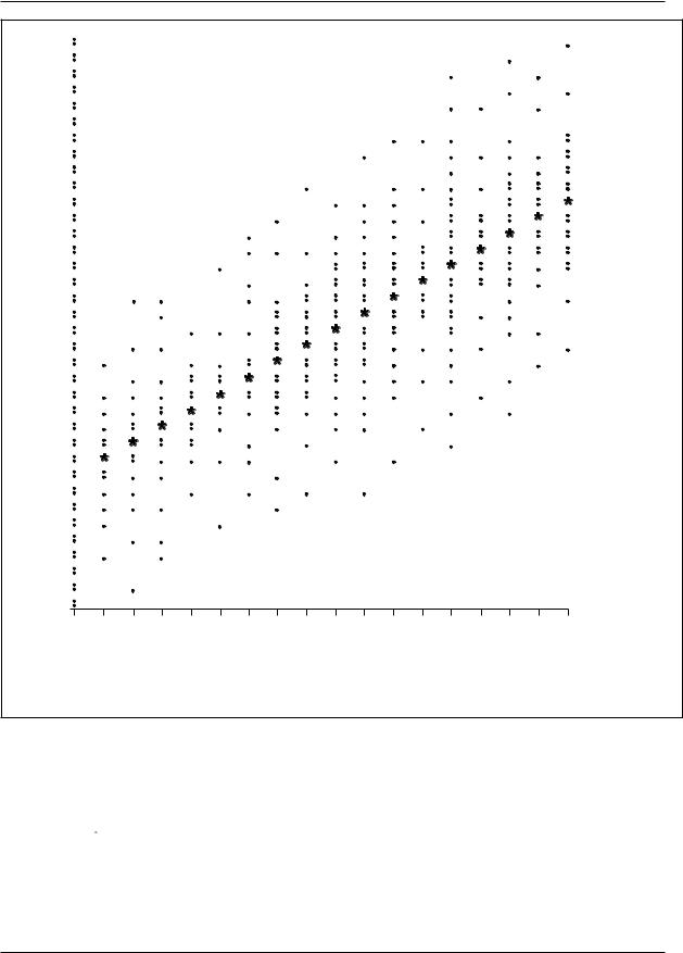
Imagine now an ordered arrangement of the subsets from left to right according to the years of school completed, with zero years of school on the left, followed by one year of school, and so on through the maximum number of years of school completed in this set of cases, as shown in Figure 1.

Assume that each of the |X values (i.e., the mean income for each level of education) falls on a straight line, as in Figure 1. This straight line is the regression line of Y on X. Thus the regression line of Y on X is the line that passes through the mean Y for each value of X—for example, the mean income for each educational level.

If this regression line is a straight line, as shown in Figure 1, then the income associated with each additional year of school completed is the same whether that additional year of school represents an increase, for example, from six to seven years of school completed or from twelve to thirteen years. While one can analyze curvilinear regression, a straight regression line greatly simplifies the analysis. Some (but not all) curvilinear regressions can be made into straight-line regressions by a relatively simple transformation of one of the variables (e.g., taking a logarithm). The common assumption that the regression line is a straight line is known as the assumption of rectilinearity, or more commonly (even if less precisely) as the assumption of linearity.

The slope of the regression line reflects one feature of the relationship between two variables.

If the regression line slopes ‘‘uphill,’’ as in Figure

1, then Y increases as X increases, and the steeper the slope, the more Y increases for each unit increase in X. In contrast, if the regression line slopes ‘‘downhill’’ as one moves from left to right, Y decreases as X increases, and the steeper the slope, the more Y decreases for each unit increase in X. If the regression line doesn’t slope at all but is perfectly horizontal, then there is no relationship between the variables. But the slope does not tell how closely the two variables are ‘‘co-related’’ (i.e., how closely the values of Y cluster around the regression line).

A regression line may be represented by a simple mathematical formula for a straight line. Thus:

where |X = the mean Y for a given value of X, or the regression line values of Y given X; ayx = the Y intercept (i.e., the predicted value of |X when X = 0); and byx = the slope of the regression of Y on X (i.e., the amount by which |X increases or de- creases—depending on whether b is positive or negative—for each one-unit increase in X).

Equation 1 is commonly written in a slightly different form:

where Ŷ = the regression prediction for Y for a given value of X, and ayx and byx are as defined above, with Ŷ substituted for |X.

Equations 1 and 2 are theoretically equivalent. Equation 1 highlights the fact that the points on the regression line are assumed to represent conditional means (i.e., the mean Y for a given X). Equation 2 highlights the fact that points on the regression line are not ordinarily found by computing a series of conditional means, but are found by alternative computational procedures.

Typically the number of cases is insufficient to yield a stable estimate of each of a series of conditional means, one for each level of X. Means based on a relatively small number of cases are inaccurate because of sampling variation, and a line connecting such unstable conditional means may not be straight even though the true regression line is. Hence, one assumes that the regression line is a straight line unless there are compelling reasons for assuming otherwise; one can then use the

X and Y values for all cases together to estimate the Y intercept, ayx, and the slope, byx, of the regression line that is best fit by the criterion of least squares. This criterion requires predicted values for Y that will minimize the sum of squared deviations between the predicted values and the observed values. Hence, a ‘‘least squares’’ regression line is the straight line that yields a lower sum of squared deviations between the predicted (regression line) values and the observed values than does any other straight line. One can find the parameters of the ‘‘least squares’’ regression line for a given set of X and Y values by computing

∑ (X – X) (Y – Y)

byx = ––––––––––––––– (3) ∑ (X – X)2

These parameters (substituted in equation 2) describe the straight regression line that best fits by the criterion of least squares. By substituting the X value for a given case into equation 2, one can then find Ŷ for that case. Otherwise stated, once ayx and byx have been computed, equation 2 will yield a precise predicted income level (Ŷ) for each education level.

These predicted values may be relatively good or relatively poor predictions, depending on whether the actual values of Y cluster closely around the predicted values on the regression line or spread themselves widely around that line. The variance of the Y values (income levels in this illustration) around the regression line will be relatively small if the Y values cluster closely around the predicted values (i.e., when the regression line provides relatively good predictions). On the other hand, the variance of Y values around the regression line will be relatively large if the Y values are spread widely around the predicted values (i.e., when the regression line provides relatively poor predictions). The

variance of the Y values around the regression predictions is defined as the mean of the squared deviations between them. The variances around each of the values along the regression line are assumed to be equal. This is known as the assumption of homoscedasticity (homogeneous scatter or variance). When the variances of the Y values around the regression predictions are larger for some values of X than for others (i.e., when homoscedasticity is not present), then X serves as a better predictor of Y in one part of its range than in another. The homoscedasticity assumption is usually at least approximately true.

The variance around the regression line is a measure of the accuracy of the regression predictions. But it is not an easily interpreted measure of the degree of correlation because it has not been

‘‘normed’’ to vary within a limited range. Two other measures, closely related to each other, provide such a normed measure. These measures, which are always between zero and one in absolute value (i.e., sign disregarded) are: (a) the correlation coefficient, r, which is the measure devised by

Karl Pearson; and (b) the square of that coefficient, r2, which, unlike r, can be interpreted as a percentage.

Pearson’s correlation coefficient, r, can be computed using the following formula:

The numerator in equation 5 is known as the covariance of X and Y. The denominator is the square root of the product of the variances of X and Y. Hence, equation 5 may be rewritten:

While equation 5 may serve as a computing guide, neither equation 5 nor equation 6 tells why it describes the degree to which two variables covary. Such understanding may be enhanced by stating that r is the slope of the least squares regression line when both X and Y have been

transformed into ‘‘standard deviates’’ or ‘‘z measures.’’ Each value in a distribution may be transformed into a ‘‘z measure’’ by finding its deviation from the mean of the distribution and dividing by the standard deviation (the square root of the variance) of that distribution. Thus

N

When both the X and Y measures have been thus standardized, ryx = rxy is the slope of the regression of Y on X, and of X on Y. For standard deviates, the Y intercept is necessarily 0, and the following equation holds:

where Ẑy = the regression prediction for the ‘‘Z measure’’ of Y, given X; Zx = the standard deviates of X; and ryx = rxy = the Pearsonian correlation between X and Y.

Like the slope byx, for unstandardized measures, the slope for standardized measures, r, may be positive or negative. But unlike byx, r is always between 0 and 1.0 in absolute value. The correlation coefficient, r, will be 0 when the standardized regression line is horizontal so that the two variables do not covary at all—and, incidentally, when the regression toward the mean, which was Galton’s original interest, is complete. On the other hand, r will be 1.0 or − 1.0 when all values of Zy fall precisely on the regression line rZx. This means that when r = + 1.0, for every case Zx = Zy—that is, each case deviates from the mean on X by exactly as much and in the same direction as it deviates from the mean on Y, when those deviations are measured in their respective standard deviation units. And when r = − 1.0, the deviations from the mean measured in standard deviation units are exactly equal, but they are in opposite directions. (It is also true that when r = 1.0, there is no regression toward the mean, although this is very rarely of any interest in contemporary applications.) More commonly, r will be neither 0 nor 1.0 in absolute value but will fall between these extremes, closer to 1.0 in absolute value when the Zy values cluster closely around the regression line, which, in this standardized form, implies that the

slope will be near 1.0, and closer to 0 when they scatter widely around the regression line.

But while r has a precise meaning—it is the slope of the regression line for standardized meas- ures—that meaning is not intuitively understandable as a measure of the degree to which one variable can be accurately predicted from the other. The square of the correlation coefficient, r2, does have such an intuitive meaning. Briefly stated, r2 indicates the percent of the possible reduction in prediction error (measured by the variance of actual values around predicted values) that is achieved by shifting from (a) as the prediction, to (b) the regression line values as the prediction.

The denominator of Equation 9 is called the total variance of Y. It is the sum of two components:

(1) the variance of the Y values around Ŷ, and (2) the variance of the Ŷ around . Hence the numerator of equation 9 is equal to the variance of the Ŷ values (regression values) around . Therefore

around Y

= proportion of variance explained

Even though it has become common to refer to r2 as the proportion of variance ‘‘explained,’’ such terminology should be used with caution. There are several possible reasons for two variables to be correlated, and some of these reasons are inconsistent with the connotations ordinarily attached to terms such as ‘‘explanation’’ or ‘‘explained.’’ One possible reason for the correlation between two variables is that X influences Y. This is presumably the reason for the positive correlation between education and income; higher education facilitates earning a higher income, and it is appropriate to refer to a part of the variation in income as being ‘‘explained’’ by variation in education. But there is also the possibility that two variables are correlated because both are measures of the same

dimension. For example, among twentieth-centu- ry nation-states, there is a high correlation between the energy consumption per capita and the gross national product per capita. These two variables are presumably correlated because both are indicators of the degree of industrial development. Hence, one variable does not ‘‘explain’’ variation in the other, if ‘‘explain’’ has any of its usual meanings. And two variables may be correlated because both are influenced by a common cause, in which case the two variables are ‘‘spuriously correlated.’’ For example, among elementa- ry-school children, reading ability is positively correlated with shoe size. This correlation appears not because large feet facilitate learning, and not because both are measures of the same underlying dimension, but because both are influenced by age. As they grow older, schoolchildren learn to read better and their feet grow larger. Hence, shoe size and reading ability are ‘‘spuriously correlated’’ because of the dependence of both on age. It would therefore be misleading to conclude from the correlation between shoe size and reading ability that part of the variation in reading ability is ‘‘explained’’ by variation in shoe size, or vice versa.

In the attempt to discover the reasons for the correlation between two variables, it is often useful to include additional variables in the analysis. Several techniques are available for doing so.

PARTIAL CORRELATION

One may wish to explore the correlation between two variables with a third variable ‘‘held constant.’’ The partial correlation coefficient may be used for this purpose. If the only reason for the correlation between shoe size and reading ability is because both are influenced by variation in age, then the correlation should disappear when the influence of variation in age is made nil—that is, when age is held constant. Given a sufficiently large number of cases, age could be held constant by considering each age grouping separately—that is, one could examine the correlation between shoe size and reading ability among children who are six years old, among children who are seven years old, eight years old, etc. (And one presumes that there would be no correlation between reading ability and shoe size among children who are homogeneous in age.) But such a procedure requires a relatively large number of children in each age grouping.

Lacking such a large sample, one may hold age constant by ‘‘statistical adjustment.’’

To understand the underlying logic of partial correlation, one considers the regression residuals (i.e., for each case, the discrepancy between the regression line value and the observed value of the predicted variable). For example, the regression residual of reading ability on age for a given case is the discrepancy between the actual reading ability and the predicted reading ability based on age. Each residual will be either positive or negative (depending on whether the observed reading ability is higher or lower than the regression prediction). Each residual will also have a specific value, indicating how much higher or lower than the agespecific mean (i.e., regression line values) the reading ability is for each person. The complete set of these regression residuals, each being a deviation from the age-specific mean, describes the pattern of variation in reading abilities that would obtain if all of these schoolchildren were identical in age.

Similarly, the regression residuals for shoe size on age describe the pattern of variation that would obtain if all of these schoolchildren were identical in age. Hence, the correlation between the two sets of residuals—(1) the regression residuals of shoe size on age and (2) the regression residuals of reading ability on age—is the correlation between shoe size and reading ability, with age ‘‘held constant.’’ In practice, it is not necessary to find each regression residual to compute the partial correlation, because shorter computational procedures have been developed. Hence,

where rxy z; = the partial coefficient between X and Y, holding Z constant; rxy = the bivariate correlation coefficient between X and Y; rxz = the bivariate correlation coefficient between X and Z; and ryz = the bivariate correlation coefficient between Y and Z.

It should be evident from equation 11 that if Z is unrelated to both X and Y, controlling for Z will yield a partial correlation that does not differ from the bivariate correlation. If all correlations are positive, each increase in the correlation between the control variable, Z, and each of the focal

variables, X and Y, will move the partial, rxy.z, closer to 0, and in some circumstances a positive

bivariate correlation may become negative after controlling for a third variable. When rxy is positive and the algebraic sign of ryz differs from the sign of rxz (so that their product is negative), the partial will be larger than the bivariate correlation, indicating that Z is a suppressor variable—that is, a variable that diminishes the correlation between X and Y unless it is controlled. Further discussion of partial correlation and its interpretation will be found in Simon 1954; Mueller, Schuessler, and Costner 1977; and Blalock 1979.

Any correlation between two sets of regression residuals is called a partial correlation coefficient. The illustration immediately above is called a first-order partial, meaning that one and only one variable has been held constant. A second-order partial means that two variables have been held constant. More generally, an nth-order partial is one in which precisely n variables have been ‘‘controlled’’ or held constant by statistical adjustment.

When only one of the variables being correlated is a regression residual (e.g., X is correlated with the residuals of Y on Z), the correlation is called a part correlation. Although part correlations are rarely used, they are appropriate when it seems implausible to residualize one variable. Generally, part correlations are smaller in absolute value than the corresponding partial correlation.

MULTIPLE REGRESSION

Earned income level is influenced not simply by one’s education but also by work experience, skills developed outside of school and work, the prevailing compensation for the occupation or profession in which one works, the nature of the regional economy where one is employed, and numerous other factors. Hence it should not be surprising that education alone does not predict income with high accuracy. The deviations between actual income and income predicted on the basis of education are presumably due to the influence of all the other factors that have an effect, great or small, on one’s income level. By including some of these other variables as additional predictors, the accuracy of prediction should be increased. Otherwise stated, one expects to predict Y better using both

X1 and X2 (assuming both influence Y) than with either of these alone.

A regression equation including more than a single predictor of Y is called a multiple regression equation. For two predictors, the multiple regression equation is:

where Ŷ = the least squares prediction of Y based

on X1 and X2; ay.12 = the Y intercept (i.e., the predicted value of Y when both X1 and X2 are 0);

by1.2 = the (unstandardized) regression slope of Y

on X1, holding X2 constant; and by2.1 = the (unstandardized) regression slope of Y on X2,

holding X1 constant. In multiple regression analysis, the predicted variable (Y in equation 12) is commonly known as the criterion variable, and the X’s are called predictors. As in a bivariate regression equation (equation 2), one assumes both rectilinearity and homoscedasticity, and one finds

the Y intercept (ay.12 in equation 12) and the regression slopes (one for each predictor; they are

by1.2 and by2.1 in equation 12) that best fit by the criterion of least squares. The b’s or regression

slopes are partial regression coefficients. The correlation between the resulting regression predictions

(Ŷ) and the observed values of Y is called the multiple correlation coefficient, symbolized by R.

In contemporary applications of multiple regression, the partial regression coefficients are typically the primary focus of attention. These coefficients describe the regression of the criterion variable on each predictor, holding constant all other predictors in the equation. The b’s in equation 12 are unstandardized coefficients. The analogous multiple regression equation for all variables expressed in standardized form is

where Ẑ = the regression prediction for the ‘‘z measure’’ of Y, given X1 and X2 Z1 = the standard

deviate of X1 Z2= the standard deviate of X2 b*y1.2 = the standardized slope of Y on X1, holding X2

constant; and b*y2.1 = the standardized slope of Y on X2, holding X1 constant.

The standardized regression coefficients in an equation with two predictors may be calculated from the bivariate correlations as follows:

where b*y1.2 = the standardized partial regression coefficient of Y on X1, controlling for X2; and b*y2.1 = the standardized partial regression coefficient of Y on X2, controlling for X1.

Standardized partial regression coefficients, here symbolized by b* (read ‘‘b star’’), are frequently symbolized by the Greek letter beta, and they are commonly referred to as ‘‘betas,’’ ‘‘beta coefficients,’’ or ‘‘beta weights.’’ While this is common usage, it violates the established practice of using Greek letters to refer to population parameters instead of sample statistics.

A comparison of equation 14, describing the standardized partial regression coefficient, b*y1.2, with equation 11, describing the partial correla-

tion coefficient, ry1.2, will make it evident that these two coefficients are closely related. They

have identical numerators but different denominators. The similarity can be succinctly expressed by

If any one of the quantities in equation 16 is 0, all are 0, and if the partial correlation is 1.0 in absolute value, both of the standardized partial regression coefficients in equation 16 must also be 1.0 in absolute value. For absolute values between 0 and

1.0, the partial correlation coefficient and the standardized partial regression coefficient will have somewhat different values, although the general interpretation of two corresponding coefficients is the same in the sense that both coefficients represent the relationship between two variables, with one or more other variables held constant. The difference between them is rather subtle and rarely of major substantive import. Briefly stated, the partial correlation coefficient—e.g., ry1.2—is the regression of one standardized residual on another standardized residual. The corresponding standardized partial regression coefficient, b*y1.2, is the regression of one residual on another, but the residuals are standard measure discrepancies from standard measure predictions, rather than the

residuals themselves having been expressed in the form of standard deviates.

A standardized partial regression coefficient can be transformed into an unstandardized partial regression coefficient by

where by1.2 = the unstandardized partial regres-

sion coefficient of Y on X1, controlling for X2; by2.1

= the unstandardized partial regression coefficient

of Y on X2, controlling for X1; b*y2.1 and b*y2.1 are standardized partial regression coefficients, as de-

fined above; sy = the standard deviation of Y; s1 = the standard deviation of X1; and s2 = the standard deviation of X2.

Under all but exceptional circumstances, standardized partial regression coefficients fall between

−1.0 and +1.0. The relative magnitude of the standardized coefficients in a given regression equation indicates the relative magnitude of the relationship between the criterion variable and the predictor in question, after holding constant all the other predictors in that regression equation. Hence, the standardized partial regression coefficients in a given equation can be compared to infer which predictor has the strongest relationship to the criterion, after holding all other variables in that equation constant. The comparison of unstandardized partial regression coefficients for different predictors in the same equation does not ordinarily yield useful information because these coefficients are affected by the units of measure. On the other hand, it is frequently useful to compare unstandardized partial regression coefficients across equations. For example, in separate regression equations predicting income from education and work experience for the United States and Great Britain, if the unstandardized regression coefficient for education in the equation for Great Britain is greater than the unstandardized regression coefficient for education in the equation for the United States, the implication is that education has a greater influence on income in Great Britain than in the

United States. It would be hazardous to draw any such conclusion from the comparison of standardized coefficients for Great Britain and the United