Chapter 4 MESHING WITH THE TRIMMING METHOD

The model at the beginning of this tutorial can be resumed from file: save_es-ice.1-valves

The following tutorial data files are used in this chapter:

TRIMMING_TUTORIALS/vlift01.dat (Valve 1 lift profile)

TRIMMING_TUTORIALS/vlift02.dat (Valve 2 lift profile)

PANELS/training.pnl

The model in this tutorial has been intermittently saved to file: save_es-ice.2-beforetrim save_es-ice.3-starsetup

An es-ice mesh can be generated using the more recent Trimming method or the original Mapping method. This chapter covers the former, a method employing trimmed-cell technology as implemented in the pro-STAR AutoMesh module. This method involves cutting a mesh template to the geometry surface and thus reducing the time and skill required to use the Mapping method (see Chapter 20 of this volume).

Note that the Trimming method requires a closed surface where separate surfaces must be connected. For some CAD models, it is necessary to define new surfaces that close the volume; for example, where you intend to apply flow boundary conditions.

The process of meshing via the Trimming method can be divided into six steps:

1. Modifying special cell sets in the geometry

2. Creating the 2D base template

3. Creating the 3D template

4. Trimming the 3D template to the geometry

5. Assembling the trimmed template

6. Running Star Setup

Modifying Special Cell Sets in the Geometry

In going through the following steps, you will use the example training panel to issue appropriate commands instead of typing them into es-ice (see Chapter 2, “User panels” in the User Guide).

To open the training panel:

•From the menu bar, select Panels > Directory

•Enter the directory location of the supplied user panel (training.pnl)

•From the menu bar, select Panels > training

In this section, you will modify some special, numbered cell sets in order to define certain geometry surfaces. This task requires you to collect various groups of surface shells into the current cell set and then save them into one of three pre-defined geometry cell sets.

To see a list of these sets:

•In the Plot Tool, activate the Geometry window from the drop-down menu

•From the menu bar, select Sets > CSet > List to display the list shown in

Figure 4-1

Figure 4-1 List of special cell sets

The ID number of these sets appears under the Set column, with CSet 0 as the currently active cell set. An “L” to the left of the ID number denotes a locked cell set. Locking cell sets helps prevent accidental modifications. The number of cells in each set appears under the Count column. To the right of this column is a label identifying the cell set (for CSet 0, the label shows the minimum and maximum cell ID numbers).

First, you must save the geometry shells of the cylinder wall to Geometry CSet 1. For symmetric models, such as this one, Geometry CSet 1 also includes the shells on the symmetry plane. Then you must save the piston shells to Geometry CSet 2 and finally the trimming surface to Geometry CSet 3. Note that the trimming shells include all the geometry surface shells and line cells resulting from the STAR-CCM+ surface preparation. However, they exclude the valves as these were modelled in the tutorial of Chapter 3 and are already available for trimming.

To define the geometry cell sets:

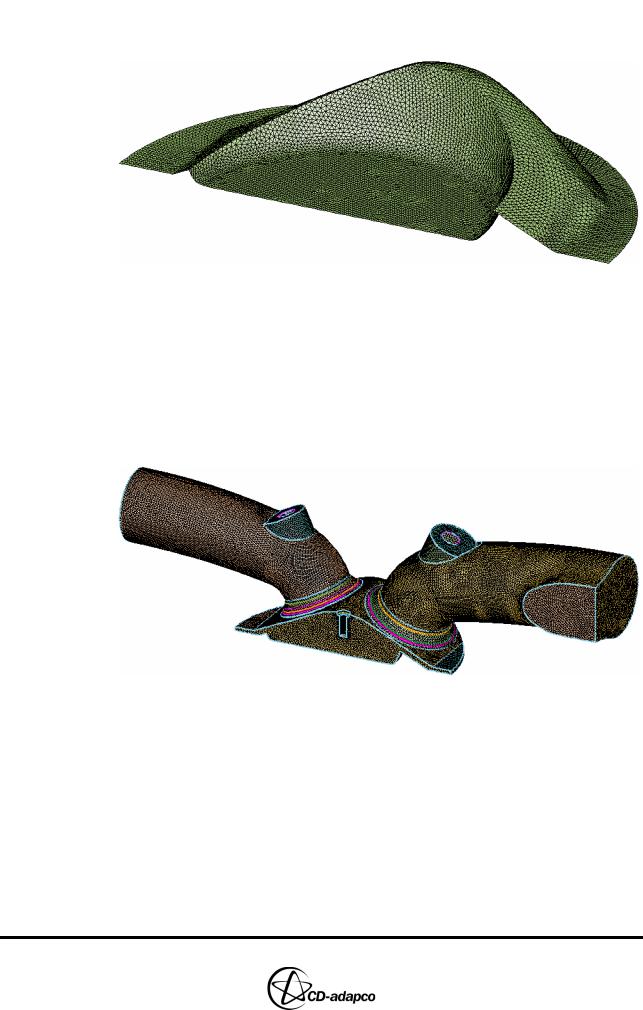
•Enter the following command to isolate the cylinder shells shown in Figure 4-2

CSet, Newset, Name, Liner

•In the training panel, click Cylinder Shells to save the cylinder wall shells into CSet 1

Figure 4-2 Cylinder shell selection

•Enter the following command to isolate the piston shells shown in Figure 4-3

CSet, Newset, Name, Piston

Figure 4-3 Piston shell selection

•Enter the following commands to isolate the trimming shells shown in Figure 4-2

CSet, All

CSet, Delete, Name, Valve1 CSet, Delete, Name, Valve2

•In the training panel, click Trimming Shells

Figure 4-4 Trimming shell selection

Defining Flow Boundaries

In this section, you define the shells representing boundaries where flow enters or leaves the solution domain. When trimming the model, the flow boundaries receive extruded cell layers that improve solution robustness.

To define the flow boundaries:

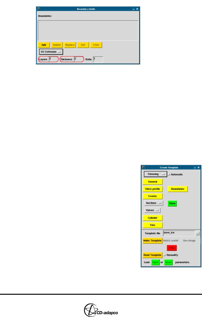
•In the Create Template panel, click Boundaries

•In the Boundary shells panel, set Layers to 2 and Thickness to 2 as shown in Figure 4-5

Figure 4-5 Boundary shells panel

•Enter the following command to isolate the Intake flow boundary:

CSet, Newset, Name, Intake

•Click Add

•Enter the following command to isolate the Exhaust flow boundary:

CSet, Newset, Name, Exhaust

•Click Add

Creating the 2D Base Template

The first step in creating the 2D base template is to define the engine operating conditions and characteristics in the General parameters and Events parameters panels.

To set the general parameters:

•In the Select panel, click Create Template

•In the Create Template panel, click General

•In the General parameters panel, set Base style to 2/4 Valve to model one half of a symmetric 4-valve engine

•Check that Engine type is Gasoline and the Cylinder radius is 45 (see Figure 4-6). All other parameters in this panel are not used for the Trimming method

•Click Ok to accept the current settings and close the panel

The starting crank angle is the 0-lift point before the valve begins to move (see vlift01.dat) and the engine speed is 3600 RPM.

To set the corresponding STAR “events” parameters:

•In the Create Template panel, click Events

•In the Events parameters panel, set Crank angle start (deg) to 320 and Crank angle stop (deg) to 1080

•Set Engine RPM to 3600

•Check that the Connecting rod length is 145, the Piston pin offset is 0 and the Valve lift periodicity (deg) is 720 (see Figure 4-6)

•Click Ok

Figure 4-6 Modified General parameters and Events parameters panels

Next, you must create a 2D base template for Valve 1. This procedure requires setting parameters in the Section Tool panel to define the cell count in certain parts of the template. For definitions and illustrations of this panel’s parameters see Chapter 4, “The Section Tool panel and the Section Adjustment points” in the User Guide. You should then manually adjust the mesh in the Workspace window to improve the cell distribution and quality.

To begin creating the 2D template for Valve

1:

•In the Create Template panel, select Section 1 from the Sections pull-down menu

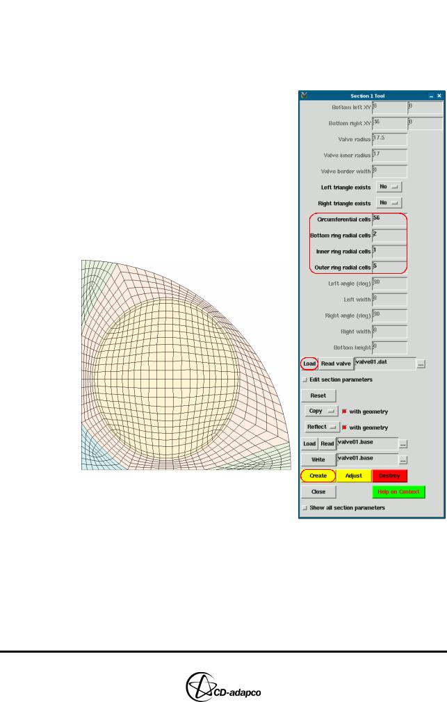
•In the Section 1 Tool panel, click the upper Load button located next to the valve01.dat field to load the internal valve information for Valve 1

•Click Create to activate the General Workspace window and plot the section, as shown in Figure 4-7

Figure 4-7 Section 1 after loading the valve information

You can reduce the cell count to reduce processing times, but a coarse mesh compromises the solution accuracy. However, as this tutorial presents a simplified case, a low cell count is acceptable. The cell density in the valve region is a major factor affecting the overall cell count of the model. You can control the mesh density in this region by adjusting the number of circumferential cells around the valve.

To reduce the cell count:

•In the Section 1 Tool, set Circumferential cells to 56

•To see the result of this modification, click Create in the Section 1 Tool panel

For most mesh adjustments, it is easier and more intuitive to use the cursor in interactive graphics mode.

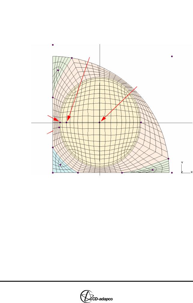
•In the Section 1 Tool, click Adjust and notice that several adjustment points appear in the Workspace window, as shown in Figure 4-8.

Adjusts “Bottom ring radial cells”

Adjusts number of circumferential cells around valve

Adjusts “Inner ring radial cells”

Adjusts “Outer ring radial cells”

Figure 4-8 Section 1 in ‘Adjust’ mode

You can now use interactive GUI tools to alter the section until a mesh of reasonable cell size and quality is created. Note the text at the bottom of the Workspace window when moving the cursor over one of the adjustment points.

•A left-click or middle-click decreases or increases, respectively, the value by 2

•A right-click resets the value to the default of 72

•Typing a number before a left-click or middle-click decreases or increases, respectively, the value by that typed number

•Typing u or r performs an “undo” or “redo”, respectively

•Clicking with any mouse button on an empty part of the window or typing q quits the ‘Adjust’ mode

The valve mesh is known as an O-grid, being made up of a 12x12 Cartesian mesh with a one-layer polar mesh surrounding it. This polar mesh is called the “Bottom ring radial cells”. The adjustment point that is associated with this parameter is

located along the mesh line of the core Cartesian grid. The default value of 2 provides adequate quality in the outer cells on this grid.

However, you need to coarsen the polar mesh around the valve region, called the “Outer ring radial cells”:

•Click twice over the adjustment point labelled “Outer ring radial cells” in Figure 4-8 to decrease it from the default value of 5 to 3

•Accept the default value of 1 for the “Inner ring radial cells”

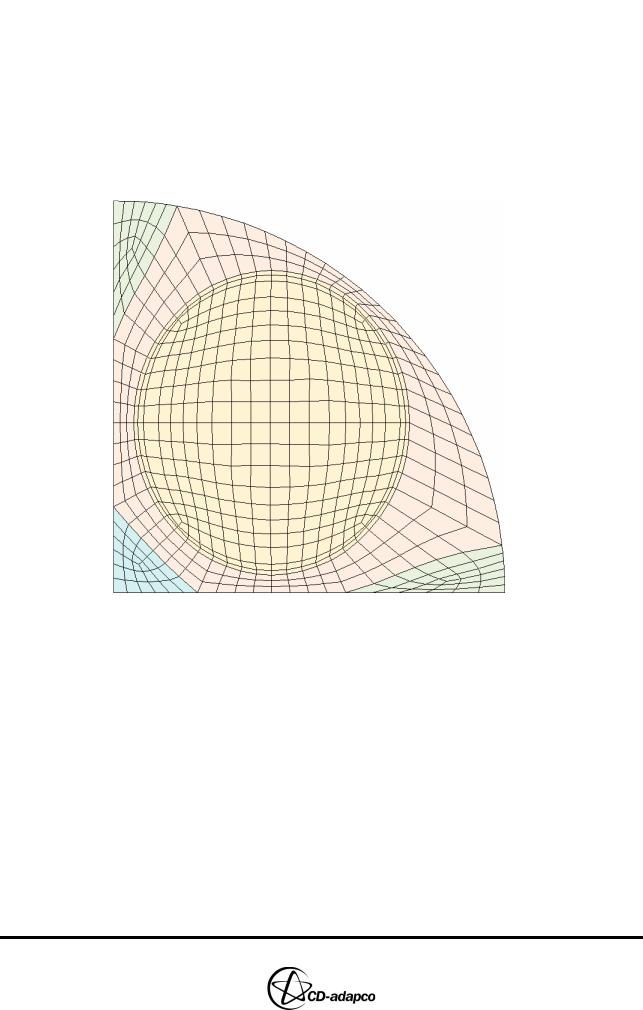
The 2D template at this stage is shown in Figure 4-9

Figure 4-9 Section 1 after valve modifications

If possible, attempt to match some areas of the 2D base template with features on the cylinder dome. For this example, there is a feature between the flat and angled portions of the combustion dome (squish region) that can be matched with a mesh line in Section 1. This line can be obtained by adding a special triangular region to the section. From the current viewpoint of looking down along the +z axis, this geometric feature appears to the right of Valve 1.

In the following steps, you will employ the ‘double-plotting’ feature by overlaying both the Geometry and General Workspace windows using the suggested plot settings of Figure 4-10:

•In the Plot Tool, activate the Geometry window from the drop-down menu

•In the Geometry window, enter the following command to isolate the cylinder dome cells

CSet, Newset, Name, Head

•In the Plot Tool, deselect the Mesh toggle button

•Activate the Workspace window

•In the Plot Tool, deselect the Fill toggle button

•Click DPlot to plot the display in the Workspace window over the display in the Geometry window

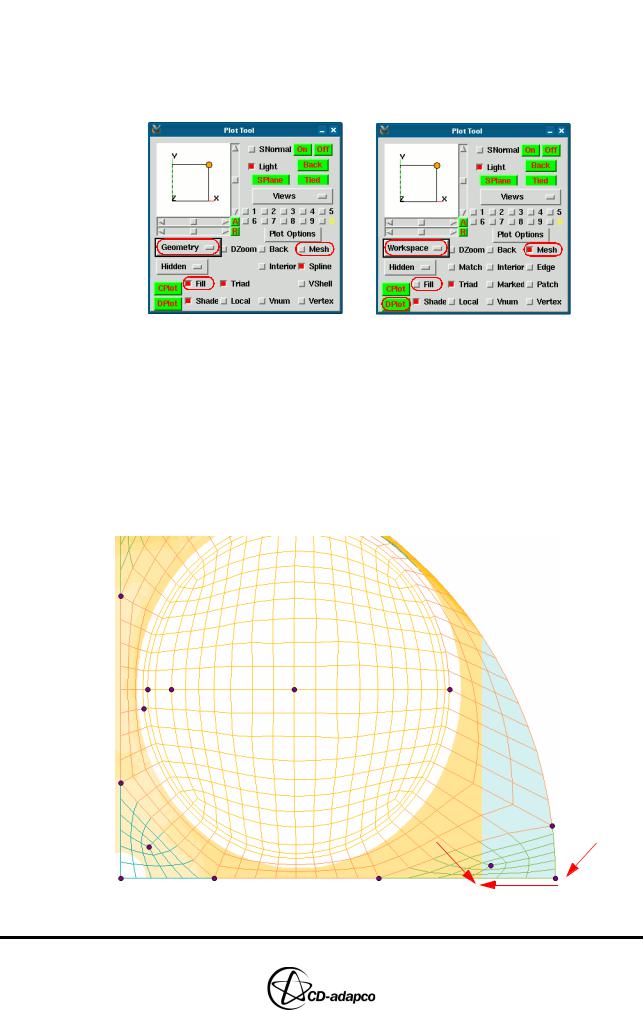
Figure 4-10 Plot Tool settings for double-plotting

As a result of the difference in colours on the cylinder dome, the feature between the flat and angled portions of the dome appears as a vertical line.

•In the Section 1 Tool, click Adjust

•Click the adjustment point on the lower-right corner to select the bottom position

•Click the previously mentioned feature to move the vertical mesh line along the bottom edge of the x-axis to the new parallel position, as shown in Figure 4-11

Figure 4-11 DPlot: Adjusting the right-bottom position

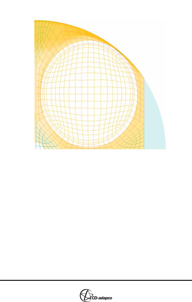
The right-hand boundary of the section has moved to match the feature, as shown in Figure 4-12

Figure 4-12 DPlot: After the right-bottom adjustment

Next, you must create a new triangular region to the right of the 2D template, as shown in Figure 4-13, using the Right triangle exists parameter. Note that with Right triangle exists activated, further adjustment of the vertical mesh line will also automatically adjust the newly created triangular region.

To create a triangular region on the right-hand side of the 2D template:

•In the Section 1 Tool, set the Right triangle exists option to Yes

•Click Create

•In the Plot Tool panel, select the Fill option and then click CPlot

Figure 4-13 2D Template after using the Right triangle exists option

Other important areas for modification are the three triangular regions at the corners of the section. There are two issues with these regions:

1.The placement of the corner attachment points

2.The cell density within the regions

To address these issues, begin by modifying the mesh as follows:

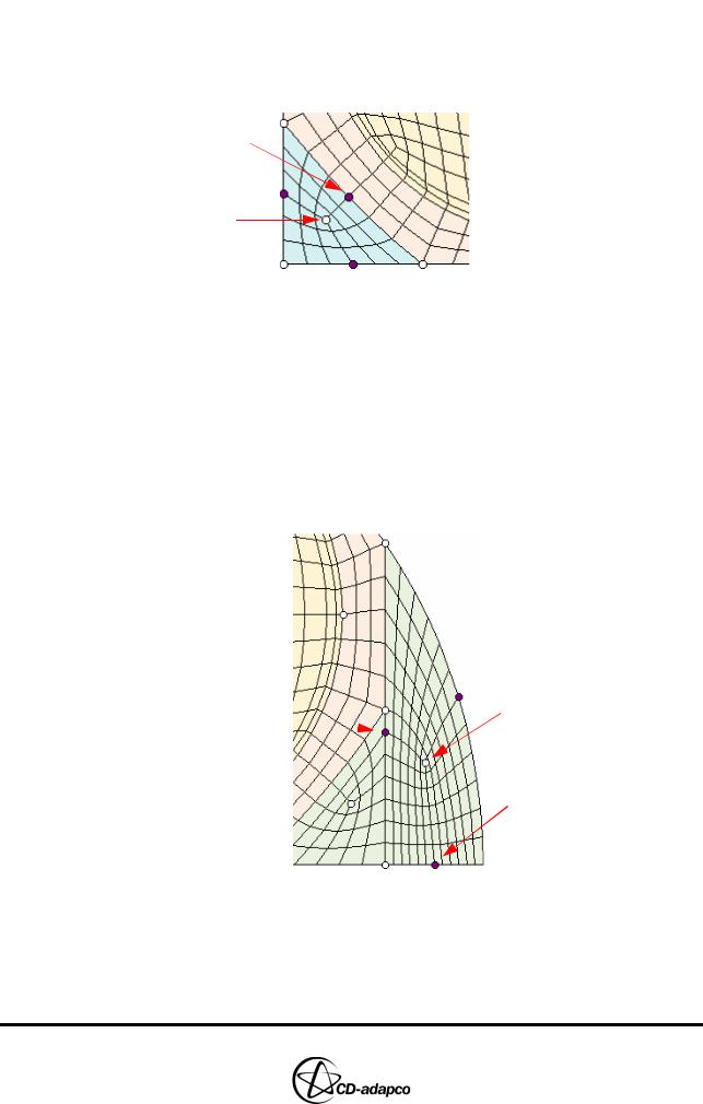
•Move the cursor over the upper adjustment point of the “Right triangle” region, as shown in Figure 4-14, and note the text at the bottom of the window

•Left-click to choose this point for adjustment. All other adjustment points become clear and the text changes to:

•Left-click the vertex that is two positions away in the clockwise direction, as shown in Figure 4-14

1. Click to choose

2. Click to choose new attachment point

Figure 4-14 Adjusting the attachment point of the right triangle

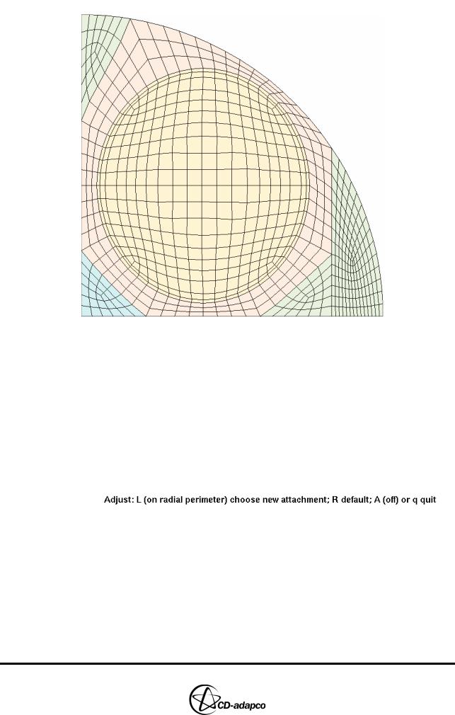
Notice the improvement in the interior angles connected to the new adjustment point and the improved mesh orthogonality in the region outside the valve and closest to the cylinder wall.

Similar improvements can be made by repeating the previous steps for the other three triangular regions:

•For the triangular region in the lower-right corner, move the top adjustment point counter-clockwise by one position, as shown in Figure 4-15

Figure 4-15 Adjusting the attachment point of the lower-right triangle

•For the triangular region in the upper-left corner, move the right adjustment point clockwise by four positions, as shown in Figure 4-16

Figure 4-16 Adjusting the attachment point of the upper-left triangle

The previous operations result in greater cell size uniformity in the “Outer ring radial cells” region, as shown in Figure 4-17.

Figure 4-17 Workspace window: Section 1 after attachment point adjustments

Since the spark plug is located in the triangular region on the lower-left corner of Section 1, increasing the cell density in this region improves the solution accuracy. You can control the cell density of the triangular region by increasing or decreasing the number of cell layers from the centre to each of the three edges.

•Click the adjustment point in the centre of this triangular region and note the text at the bottom of the plotting window (see Figure 4-18). Notice the three adjustment points in the middle of each edge of the triangular region and the change in the text

•Middle-click the adjustment point in the interior of the section twice to add two additional cell layers between the centre and the corresponding edge

•Finish the triangular region adjustment by clicking off the mesh or typing q on the keyboard

2. Middle-click

twice to increase by 2

1. Left-click to choose

Figure 4-18 Changing the cell count within the bottom-left triangular region

Use a similar technique to reduce the cell count in the “Right triangle” region:

•Left-click the adjustment point in the centre of this region to select it

•Middle-click the bottom adjustment point four times to increase the number of cells from that edge to the centre. This adjustment decreases the overall cell count in the region

•Middle-click the left adjustment point once to increase the number of cells from that edge to the centre

•Finish the region adjustment by clicking off the mesh or typing q on the keyboard

Figure 4-19 Changing the cell count within the right triangular region

Section 1 now has an acceptable cell distribution and quality, shown in Figure 4-20.

Figure 4-20 Workspace window: Final Section 1

Section 2 can be built in a similar way. Typically, the exhaust valve is smaller than the intake valve and therefore needs fewer circumferential cells. However, you should use more “Outer ring radial cells” than the intake valve section to maintain a consistent cell spacing.

As Valve 2 is a recessed valve, you can specify a few extra parameters to capture this feature accurately in the 2D template. Inspection of the geometry reveals an axisymmetric “step” feature that is at a radial distance of 16.5 millimetres in the local valve coordinate system. You can force the outer radial cell layer nearest to the valve to be a concentric ring of cells with a radial cell length of 1 millimetre. When creating Section 2, you must set the inner and outer circular mesh lines to be at a radial distance of 15.5 and 16.5 millimetres from the centre of the valve. Forcing this outer mesh line to coincide with the geometric feature of the recessed valve results in a better trimmed mesh.

To begin defining the 2D template for Valve

2:

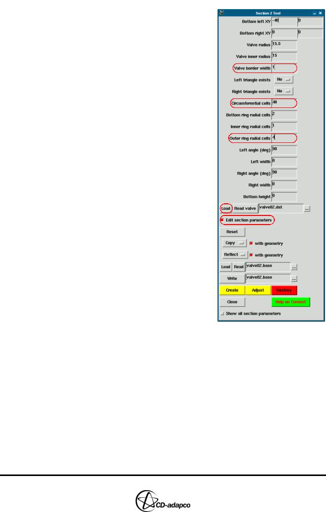
•In the Create Template panel, select Section 2 from the Sections drop-down menu

•In the Section 2 Tool, click Load to load the valve data

•Set Circumferential cells to 48

•Set Outer ring radial cells to 4

•Click the Edit section parameters button in the Section 2 Tool panel to allow direct access to additional parameters

•Note that he valve radius is 15.5

millimetres, so change the Valve border width to 1 to model the valve recess

•Accept the remaining defaults and click Create to display Section 2

The attachment points and cell densities of the triangular regions can be adjusted in a similar manner to Section 1.

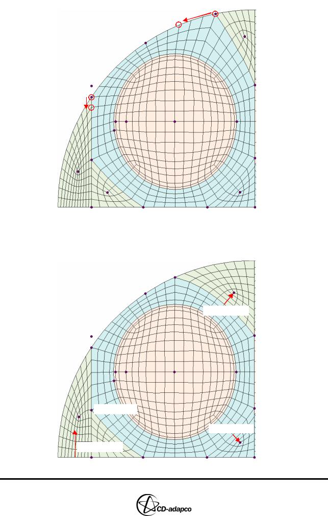
•Using similar techniques to Section 1, adjust the cells in Section 2 as follows:

•Move the bottom-right adjustment point to coincide with the geometry feature on the cylinder head

•Set Left triangle exists to Yes

•Move the attachment points to improve cell orthogonality, as shown in Figure 4-21

Figure 4-21 Moving attachment points for Section 2

•Modify the cell count to reduce cell density and match the number of cells at the interface between Section 1 and Section 2, as shown in Figure 4-22

Add 2 Layers

Add 1 Layer

Add 3 Layers

Add 3 Layers

Figure 4-22 Modifying the cell count for Section 2

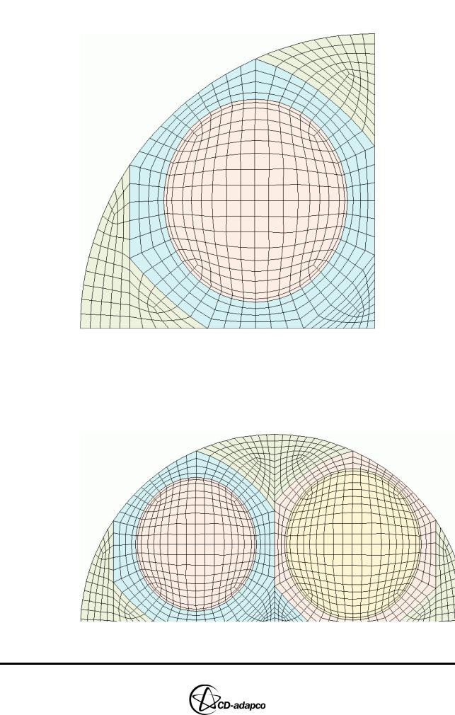
Figure 4-23 shows the completed 2D template for Section 2.

Figure 4-23 Workspace window: Final Section 2

Following every modification, the es-ice window updates the number of cells on each side of the shared interface. Only when they are equal are you able to continue.

•In the Create Template panel, click Store to smooth the mesh and connect the two sections together, as shown in Figure 4-24

Figure 4-24 Workspace window: Completed 2D base template