Creating an Animation of Temperature Isosurfaces

Figure 9-9 Fuel distribution at 400 degrees CA

Figure 9-10 shows the fuel distribution following combustion at 725 degrees CA.

Figure 9-10 Fuel distribution at 725 degrees CA

Creating an Animation of Temperature Isosurfaces

This section provides an example of how a pro-STAR input file (isoTemp.inp)

can be used to create an animation of temperature isosurfaces throughout the simulation. Opening the input file with a text editor will display its contents as shown below. For clarity, the full command names are shown, although the usual four-letter abbreviations can be used instead.

•Connect the events file and load the transient data

RESUME, , EVFILE, CONNECT TRLOAD, ,

•Create a custom colour table for use with the colour scale

CLRTABLE, POST, 1, 1.0, 0.0, 0.0, 0.3 CLRTABLE, POST, 2, 1.0, 0.6, 0.0, 0.3 CLRTABLE, POST, 3, 1.0, 1.0, 0.0, 0.3

•Specify a 20-colour scale with a user-defined value range of 2200 and 2600

CSCALE, 3, USER, 2200, 2600

•Set up the display items

PLLOCALCOOR, OFF, ALL PLDISPLAY, OFF, ALL PLDISPLAY, ON, LOGO PLDISPLAY, ON, HEAD PLDISPLAY, ON, MINMAX PLDISPLAY, ON, SCALE, ,8

•Select the Extended Graphics option and a 1024 x 768 resolution for the image

TERMINAL, , EXTENDED HRSDUMP, IMAGE, 1024, 768

•Set up a variable, it, that will be incremented at each loop iteration and begin the loop definition

*SET, it, 1, 1 *DEFINE, NOEXECUTE

•Store the next time step

STORE, NEXT

•Set up a crank-angle display label in the lower-right corner of the screen

*GET, TIME, time

*SET, CRANK, 3600 * TIME * 6 + 320 TSCALE, 4, 15

PLLABEL, 1, FORMAT, , 4, 10, 0.5 CRANK

F6.1, ' degCA'

•Remove all manifolds from the cell set and define the current cell type as no. 501

CSET, ALL

CSET, DELETE, TYPE, 121 CSET, DELETE, TYPE, 122 CTABLE, 501, FLUID CMODIFY, CSET

•Collect cell type 501 into a set and merge vertices for a clear view of the results

CSET, NEWSET, TYPE, 501 VSET, NEWSET, CSET VMERGE, VSET

•Plot cell-averaged temperature data

GETCELL, T, ABSOLUTE CAVERAGE, CSET

•Plot an isosurface at 2600 K and create a pro-STAR “layer” (described in Chapter 4 of the STAR-CD Post-Processing User Guide)

POPTION, ISOSURFACE, 2600 CPLOT

LAYER, ISO1, STORE LAYER, ISO1, HIDE

•Plot an isosurface at 2400 K and create another layer

POPTION, ISOSURFACE, 2400 CPLOT

LAYER, ISO2, STORE LAYER, ISO2, HIDE

•Plot an isosurface at 2200 K and create a third layer

POPTION, ISOSURFACE, 2400 CPLOT

LAYER, ISO2, STORE LAYER, ISO2, HIDE

•Show all layers

LAYER, ALL, SHOW

•Display the geometry edges

PLMESH, OFF CPLOT

EDGE, ON

REPLOT

•Create a counter for the file names

*SET, itn, 1000 + it *SCOPY, itn, sitn, i4

•Redisplay the mesh front view using the bottom-left corner of the graphics window and save it to a .gif file

WINDOW, 0, 0, 5, 5 VIEW, 0, -1, 0 ANGLE, 0 DISTANCE, 100 CENTER, 0, 0, -20

*SSET, sname, image_1_{sitn} HRSDUMP, GIF, {sname}

•Redisplay the mesh side view using the bottom-right corner of the graphics window and save it to a .gif file

WINDOW, 5, 0, 10, 5 VIEW, 1, 0, 0 ANGLE, 0

DISTANCE, 100 CENTER, 20, 20, -20

*SSET, sname, image_2_{sitn} HRSDUMP, GIF, {sname}

•Redisplay an isometric view of the mesh using the top-right corner of the graphics window and save it to a .gif file

WINDOW, 5, 5, 10, 10 VIEW, 1, 1, -1 ANGLE, 0

DISTANCE, 115 CENTER, -5, 10, -25

*SSET, sname, image_3_{sitn} HRSDUMP, GIF, {sname}

•Redisplay the mesh top view using the top-left corner of the graphics window and save it to a .gif file

WINDOW, 0, 5, 5, 10 VIEW, 0, 0, 1 ANGLE, -90 DISTANCE, 100.0 CENTER, 0, 20, -20

*SSET, sname, image_4_{sitn} HRSDUMP, GIF, {sname}

•End the loop definition and then execute the loop for all time steps

*END

*LOOP, 0, 152

image_2_${i}t.gif

convert image_3_${i}.gif -transparent \#ffffff image_3_${i}t.gif

convert image_4_${i}.gif -transparent \#ffffff image_4_${i}t.gif

done

for (( i=1001; $i <= ${sum}; i++ )) do

composite -compose atop image_2_${i}t.gif image_1_${i}.gif comp1_${i}.gif

composite -compose atop image_3_${i}t.gif comp1_${i}.gif comp2_${i}.gif

composite -compose atop image_4_${i}t.gif comp2_${i}.gif final_${i}.gif

done

•Remove unnecessary files rm comp*.gif *t.gif

•Create an animation file called tempIso.gif using WhirlGif gifsicle -d 10 -l -o tempIso.gif final*.gif

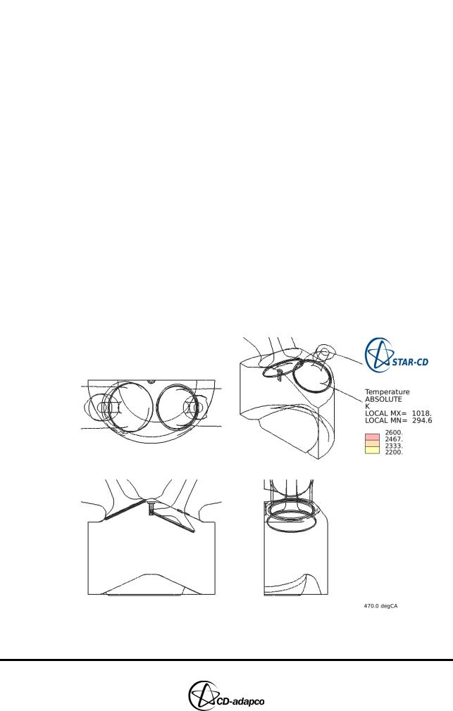
Figure 9-11 shows the intake valve fully open at 470 degrees CA.

Figure 9-11 Intake valve at 470 degrees CA

Figure 9-12 Isosurfaces at 730 degrees CA.