primer_on_scientific_programming_with_python

Another, more serious, problem is the possibility dividing by zero. Almost as serious, is dividing by a very small number that creates a large value, which might cause Newton’s method to diverge. Therefore, we should test for small values of f (x) and write a warning or raise an exception.

Another improvement is to add a boolean argument store to indicate whether we want the (x, f (x)) values during the iterations to be stored in a list or not. These intermediate values can be handy if we want to print out or plot the convergence behavior of Newton’s method.

An improved Newton function can now be coded as

def Newton(f, x, dfdx, epsilon=1.0E-7, N=100, store=False): f_value = f(x)

n = 0

if store: info = [(x, f_value)]

while abs(f_value) > epsilon and n <= N: dfdx_value = float(dfdx(x))

if abs(dfdx_value) < 1E-14:

raise ValueError("Newton: f’(%g)=%g" % (x, dfdx_value))

x = x - f_value/dfdx_value

n += 1 f_value = f(x)

if store: info.append((x, f_value)) if store:

return x, info else:

return x, n, f_value

Note that to use the Newton function, we need to calculate the derivative f (x) and implement it as a Python function and provide it as the dfdx argument. Also note that what we return depends on whether we store (x, f (x)) information during the iterations or not.

It is quite common to test if dfdx(x) is zero in an implementation of Newton’s method, but this is not strictly necessary in Python since an exception ZeroDivisionError is always raised when dividing by zero.

We can apply the Newton function to solve the equation8 e−0.1x2 sin( π2 x) = 0:

from math import sin, cos, exp, pi import sys

from Newton import Newton

def g(x):

return exp(-0.1*x**2)*sin(pi/2*x)

def dg(x):

return -2*0.1*x*exp(-0.1*x**2)*sin(pi/2*x) + \ pi/2*exp(-0.1*x**2)*cos(pi/2*x)

x0 = float(sys.argv[1])

x, info = Newton(g, x0, dg, store=True)

8Fortunately you realize that the exponential function can never be zero, so the solutions of the equation must be the zeros of the sine function, i.e., π2 x = iπ for all integers i = . . . , −2, 1, 0, 1, 2, . . .. This gives x = 2i as the solutions.

250 5 Sequences and Di erence Equations

print ’root:’, x

for i in range(len(info)):

print ’Iteration %3d: f(%g)=%g’ % \ (i, info[i][0], info[i][1])

The Newton function and this program can be found in the file Newton.py. Running this program with an initial x value of 1.7 results in the output

root: 1.999999999768449 Iteration 0: f(1.7)=0.340044

Iteration 1: f(1.99215)=0.00828786 Iteration 2: f(1.99998)=2.53347e-05 Iteration 3: f(2)=2.43808e-10

The convergence is fast towards the solution x = 2. The error is of the order 10−10 even though we stop the iterations when f (x) ≤ 10−7.

Trying a start value of 3 we would expect the method to find either nearby solution x = 2 or x = 4, but now we get

root: 42.49723316011362 Iteration 0: f(3)=-0.40657

Iteration 1: f(4.66667)=0.0981146 Iteration 2: f(42.4972)=-2.59037e-79

We have definitely solved f (x) = 0 in the sense that |f (x)| ≤ , whereis a small value (here 10−79). However, the solution x ≈ 42.5 is not close to the solution (x = 42 and x = 44 are the solutions closest to the computed x). Can you use your knowledge of how the Newton method works and figure out why we get such strange behavior?

The demo program Newton_movie.py can be used to investigate the strange behavior. This program takes five command-line arguments: a formula for f (x), a formula for f (x) (or the word numeric, which indicates a numerical approximation of f (x)), a guess at the root, and the minimum and maximum x values in the plots. We try the following case with the program:

Terminal

Newton_movie.py ’exp(-0.1*x**2)*sin(pi/2*x)’ numeric 3 -3 43

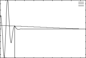
As seen, we start with x = 3 as the initial guess. In the first step of the method, we compute a new value of the root, now x = 4.66667. As we see in Figure 5.2, this root is near an extreme point of f (x) so that the derivative is small, and the resulting straight line approximation to f (x) at this root becomes quite flat. The result is a new guess at the root: x42.5. This root is far away from the last root, but the second problem is that f (x) is quickly damped as we move to increasing x values, and at x = 42.5 f is small enough to fulfill the convergence criterion. Any guess at the root out in this region would satisfy that criterion.

You can run the Newton_movie.py program with other values of the initial root and observe that the method usually finds the nearest roots.

Fig. 5.2 Failure of Newton’s method to solve e−0.1x2 sin( π2 x) = 0. The plot corresponds to the second root found (starting with x = 3).

5.1.10 The Inverse of a Function

Given a function f (x), the inverse function of f , say we call it g(x), has the property that if we apply g to the value f (x), we get x back:

g(f (x)) = x .

Similarly, if we apply f to the value g(x), we get x:

By hand, you substitute g(x) by (say) y in (5.32) and solve (5.32) with respect to y to find some x expression for the inverse function. For example, given f (x) = x2 − 1, we must solve y2 − 1 = x with respect to y. To ensure a unique solution for y, the x values have to be limited

Numerically, we can use the “definition” (5.32) of the inverse function g at one point at a time. Suppose we have a sequence of points x0 < x1 < · · · < xN along the x axis such that f is monotone in [x0, xN ]: f (x0) > f (x1) > · · · > f (xN ) or f (x0) < f (x1) < · · · < f (xN ). For each point xi, we have

f (g(xi)) = xi .

The value g(xi) is unknown, so let us call it γ. The equation

can be solved be respect γ. However, (5.33) is in general nonlinear if f is a nonlinear function of x. We must then use, e.g., Newton’s method

252 5 Sequences and Di erence Equations

to solve (5.33). Newton’s method works for an equation phrased as “f (x) = 0”, which in our case is f (γ) − xi = 0, i.e., we seek the roots of the function F (γ) ≡ f (γ) − xi. Also the derivative F (γ) is needed in Newton’s method. For simplicity we may use an approximate finite di erence:

As start value γ0, we can use the previously computed g value: gi−1. We introduce the short notation γ = Newton(F, γ0) to indicate the solution of F (γ) = 0 with initial guess γ0.

The computation of all the g0, . . . , gN values can now be expressed

by

Equations (5.34)–(5.35) constitute a di erence equation for gi, since , we can compute the next element of the sequence by (5.34).

Because (5.34) is a nonlinear equation in the new value gi, and (5.34) is therefore an example of a nonlinear di erence equation.

The following program computes the inverse function g(x) of f (x) at some discrete points x0, . . . , xN . Our sample function is f (x) = x2 −1:

from Newton import Newton from scitools.std import *

def f(x):

return x**2 - 1

def F(gamma):

return f(gamma) - xi

def dFdx(gamma):

return (F(gamma+h) - F(gamma-h))/(2*h)

h = 1E-6

x = linspace(0.01, 3, 21) g = zeros(len(x))

for i in range(len(x)): xi = x[i]

# compute start value (use last g[i-1] if possible): if i == 0:

gamma0 = x[0] else:

gamma0 = g[i-1]

gamma, n, F_value = Newton(F, gamma0, dFdx) g[i] = gamma

plot(x, f(x), ’r-’, x, g, ’b-’,

title=’f1’, legend=(’original’, ’inverse’))

Note that with f (x) = x2 − 1, f (0) = 0, so Newton’s method divides by zero and breaks down unless with let x0 > 0, so here we set x0 = 0.01. The f function can easily be edited to let the program compute the inverse of another function. The F function can remain the same since it applies a general finite di erence to approximate the derivative of the f(x) function. The complete program is found in the file inverse_function.py. A better implementation is suggested in Exercise 7.20.

5.2 Programming with Sound

Sound on a computer is nothing but a sequence of numbers. As an example, consider the famous A tone at 440 Hz. Physically, this is an oscillation of a tunefork, loudspeaker, string or another mechanical medium that makes the surrounding air also oscillate and transport the sound as a compression wave. This wave may hit our ears and through complicated physiological processes be transformed to an electrical signal that the brain can recognize as sound. Mathematically, the oscillations are described by a sine function of time:

where A is the amplitude or strength of the sound and f is the frequencey (440 Hz for the A in our example). In a computer, s(t) is represented at discrete points of time. CD quality means 44100 samples per second. Other sample rates are also possible, so we introduce r as the sample rate. An f Hz tone lasting for m seconds with sample rate r can then be computed as the sequence

With Numerical Python this computation is straightforward and very e cient. Introducing some more explanatory variable names than r, A, and m, we can write a function for generating a note:

import numpy

def note(frequency, length, amplitude=1, sample_rate=44100): time_points = numpy.linspace(0, length, length*sample_rate)

data = numpy.sin(2*numpy.pi*frequency*time_points) data = amplitude*data

return data

5.2.1 Writing Sound to File

The note function above generates an array of float data representing a note. The sound card in the computer cannot play these data, because

data = data.astype(float)

The write function automatically transforms the element type back to int16 if we have not done this explicitly.

One operation that we can easily do is adding an echo. Mathematically this means that we add a damped delayed sound, where the original sound has weight β and the delayed part has weight 1 − β, such that the overall amplitude is not altered. Let d be the delay in seconds. With a sampling rate r the number of indices in the delay becomes dr, which we denote by b. Given an original sound sequence sn, the sound with echo is the sequence

We cannot start n at 0 since e0 = s0−b = s−b which is a value outside the sound data. Therefore we define en = sn for n = 0, 1, . . . , b, and add the echo thereafter. A simple loop can do this (again we use descriptive variable names instead of the mathematical symbols introduced):

def add_echo(data, beta=0.8, delay=0.002, sample_rate=44100): newdata = data.copy()

shift = int(delay*sample_rate) # b (math symbol)

for i in range(shift, len(data)):

newdata[i] = beta*data[i] + (1-beta)*data[i-shift] return newdata

The problem with this function is that it runs slowly, especially when we have sound clips lasting several seconds (recall that for CD quality we need 44100 numbers per second). It is therefore necessary to vectorize the implementation of the di erence equation for adding echo. The update is then based on adding slices:

newdata[shift:] = beta*data[shift:] + \

(1-beta)*data[:len(data)-shift]

5.2.3 Playing Many Notes

How do we generate a melody mathematically in a computer program? With the note function we can generate a note with a certain amplitude, frequence, and duration. The note is represented as an array. Putting sound arrays for di erent notes after each other will make up a melody. If we have several sound arrays data1, data2, data3, . . ., we can make a new array consisting of the elements in the first array followed by the elements of the next array followed by the elements in the next array and so forth:

data = numpy.concatenate((data1, data2, data3, ...))

Here is an example of creating a little melody (start of “Nothing Else Matters” by Metallica) using constant (max) amplitude of all the notes:

E1 = note(164.81, .5) G = note(392, .5)

B = note(493.88, .5) E2 = note(659.26, .5)

intro = numpy.concatenate((E1, G, B, E2, B, G)) high1_long = note(987.77, 1)

high1_short = note(987.77, .5) high2 = note(1046.50, .5) high3 = note(880, .5) high4_long = note(659.26, 1) high4_medium = note(659.26, .5) high4_short = note(659.26, .25) high5 = note(739.99, .25) pause_long = note(0, .5) pause_short = note(0, .25) song = numpy.concatenate(

(intro, intro, high1_long, pause_long, high1_long, pause_long, pause_long,

high1_short, high2, high1_short, high3, high1_short, high3, high4_short, pause_short, high4_long, pause_short, high4_medium, high5, high4_short))

scitools.sound.play(song) scitools.sound.write(song, ’tmp.wav’)

We could send song to the add_echo function to get some echo, and we could also vary the amplitudes to get more dynamics into the song. You can find the generation of notes above as the function

Nothing_Else_Matters(echo=False) in the scitools.sound module.

5.3 Summary

5.3.1 Chapter Topics

Sequences. In general, a finite sequence can be written as

(xn)Nn=0, xn = f (n),

where f (n) is some expression involving n and possibly other parameters. The coding of such a sequence takes the form

x = zeros(N+1)

for n in range(N+1): x[n] = f(n)

Here, we store the whole sequence in an array, which is convenient if we want to plot the evolution of the sequence (i.e., xn versus n). Occasionally, this can require too much memory. Especially when checking for convergence of xn toward some limit as N → ∞, N may be large

if the sequence converges slowly. The array can be skipped if we print the sequence elements as they are computed:

for n in range(N+1):

print f(n)

Di erence Equations. Equations involving more than one element of a sequence are called di erence equations. We have typically looked at di erence equations relating xn to the previous element xn−1:

xn = f (xn−1),

where f is some specified function. Any di erence equation must have an initial condition prescribing x0, say x0 = X. The solution of a di erence equation is a sequence. Very often, n corresponds to a time parameter in applications.

We have also looked at systems of di erence equations of the form

xn = f (xn−1, yn−1), x0 = X yn = g(yn−1, xn−1, xn), y0 = Y

where f and g denote formulas involving already computed quantities. Note that xn does not depend on yn, which means that we can first compute xn and then yn:

index_set = range(N+1)

x = zeros(len(index_set)) y = zeros(len(index_set)) x[0] = X

y[0] = Y

for n in index_set[1:]: x[n] = f(x[n-1], y[n-1])

y[n] = g(y[n-1], x[n], x[n-1])

Sound. Sound on a computer is a sequence of 2-byte integers. These can be stored in an array. Creating the sound of a tone consist of sampling a sine function and storing the values in an array (and converting to 2-byte integers). If we want to manipulate a given sound, say add some echo, we convert the array elements to ordinary floating-point numbers and peform mathematical operations on the array elements.

5.3.2 Summarizing Example: Music of a Sequence

Problem. The purpose of this summarizing example is to listen to the sound generated by two mathematical sequences. The first one is given by an explicit formula, constructed to oscillate around 0 with decreasing amplitude:

will make a standard A reference tone out of xn = 0, and for the maximum value of xn around 1 we get a tone of 640 Hz. Elements of the sequence generated by (5.39) lie between -1 and 1, so the corresponding frequences lie between 240 Hz and 640 Hz. The task now is to make a program that can generate and play the sounds.

Solution. Tones can be generated by the note function from the scitools.sound module. We collect all tones corresponding to all the yn frequencies in a list tones. Letting N denote the number of sequence elements, the relevant code segment reads

from scitools.sound import * freqs = 440 + x*200

tones = []

duration = 30.0/N # 30 sec sound in total for n in range(N+1):

tones.append(max_amplitude*note(freqs[n], duration, 1)) data = concatenate(tones)

write(data, filename) data = read(filename) play(filename)

It is illustrating to plot the sequences too,

plot(range(N+1), freqs, ’ro’)

To generate the sequences (5.39) and (5.40), we make two functions, oscillations and logistic, respectively. These functions take the number of sequence elements (N) as input and return the sequence stored in an array.

In another function make_sound we compute the sequence, transform the elements to frequencies, generate tones, write the tones to file, and play the sound file.