

primer_on_scientific_programming_with_python
.pdf198 |
4 Array Computing and Curve Plotting |
|
|
ax = axes(viewport=[left, bottom, width, height])
The four parameteres left, bottom, width, height are location values between 0 and 1 ((0,0) is the lower-left corner and (1,1) is the upperright corner). However, this might be a bit di erent in the di erent backends (see the documentation for the backend in question).
4.3.9 Curves in Pure Text
Sometimes it can be desirable to show a graph in pure ASCII text, e.g., as part of a trial run of a program included in the program itself (cf. the introduction to Chapter 1.8), or a graph can be needed in a doc string. For such purposes we have slightly extended a module by Imri Goldberg (aplotter.py) and included it as a module in SciTools. Running pydoc on scitools.aplotter describes the capabilities of this type of primitive plotting. Here we just give an example of what it can do:
>>>from scitools.aplotter import plot
>>>from numpy import linspace, exp, cos, pi
>>>x = linspace(-2, 2, 81)
>>>y = exp(-0.5*x**2)*cos(pi*x)
>>>plot(x, y)
|
|
|
| |
|
|
|
|
|
// |\\ |
|
|
|
|
/ |
| |
\ |
|
|
|
/ |
| |
\ |
|
|
|
/ |
| |
\ |
|
|
|
/ |
| |
\ |
|
|
|
/ |
| |
\ |
|
|
|
/ |
| |
\ |
|
|
|
/ |
| |
\ |
|
------- |
\ |
/ |
| |
\ |
|
---+------- |
\\----------------- |
/--------- |
+-------- |
\----------------- |
|
-2 |
\ |
/ |
| |
\ |
/ |
|
\\ |
/ |
| |
\ |
// |
|
\ |
/ |
| |
\ |
/ |
|
\\ |
/ |
| |
\ |
// |
|
\ |
/ |
| |
\ |
/ |
|
\ |
// |
| |
\- |
// |
|
|
---- |
-0.63 |
---/ |
|
|
|
|
| |
|
|
>>># plot circles at data points only:
>>>plot(x, y, dot=’o’, plot_slope=False)
|
|
|
| |
|
|
|
|
|
o+1 |
|
|
|
|
|
oo |oo |
|
|
|
|
o |
| |
o |
|
|
|
o |
| |
o |
|
|
|
|
| |
|
|
|
|
o |
| |
o |
|
|
|
o |
| |
o |
|
|
|
|
| |
|
|
oooooooo |
|
o |
| |
o |
|
---+------- |
oo----------------- |
o--------- |
+-------- |
o----------------- |
|
-2 |
o |
|
| |
|
o |
|
oo |
o |
| |
o |
oo |

4.4 Plotting Di culties |
|
|
|
199 |
|
|
|
|
|
|
|
|
|
|
|
|
|
o |
o |
| |
o |
o |
|
oo |
o |
| |
o |
oo |
|
o |
o |
| |
o |
o |
|
o |
oo |
| |
oo |
oo |
|
|
oooo |
-0.63 |
oooo |
|
|
|
|
| |
|
|
|
>>> p = plot(x, y, output=str) |
# store plot in a string: |
|
|
||
>>> print p |
|
|
|
|
|
|
|
|
|
|
|
(The last 13 characters of the output lines are here removed to make the lines fit the maximum textwidth of this book.)
4.4 Plotting Di culties
The previous examples on plotting functions demonstrate how easy it is to make graphs. Nevertheless, the shown techniques might easily fail to plot some functions correctly unless we are careful. Next we address two types of di cult functions: piecewisely defined functions and rapidly varying functions.
4.4.1 Piecewisely Defined Functions
A piecewisely defined function has di erent function definitions in different intervals along the x axis. The resulting function, made up of pieces, may have discontinuities in the function value or in derivatives. We have to be very careful when plotting such functions, as the next two examples will show. The problem is that the plotting mechanism draws straight lines between coordinates on the function’s curve, and these straight lines may not yield a satisfactory visualization of the function. The first example has a discontinuity in the function itself at one point, while the other example has a discontinuity in the derivative at three points.
Example: The Heaviside Function. Let us plot the Heaviside function defined in (2.18) on page 108. The most natural way to proceed is first to define the function as
def H(x):
return (0 if x < 0 else 1)
The standard plotting procedure where we define a coordinate array x and do a
y = H(x)
plot(x, y)
fails with this H(x) function. The test x < 0 results in an array where each element is True or False depending on whether x[i] < 0 or not.

200 |
4 Array Computing and Curve Plotting |
|
|
A ValueError exception is raised when we use this resulting array in an if test:
>>>x = linspace(-10, 10, 5)
>>>x
array([-10., -5., 0., 5., 10.])
>>>b = x < 0
>>>b
array([ True, True, False, False, False], dtype=bool)
>>> bool(b) # evaluate b in a boolean context
...
ValueError: The truth value of an array with more than one element is ambiguous. Use a.any() or a.all()
The suggestion of using the any or all methods do not help because this is not what we are interested in:
>>>b.any() # True if any element in b is True True
>>>b.all() # True if all elements in b are True False
We want to take actions element by element depending on whether x[i] < 0 or not.
There are three ways to find a remedy to our problems with the if x < 0 test: (i) we can write an explicit loop for computing the elements, (ii) we can use a tool for automatically vectorize H(x), or (iii) we can manually vectorize the H(x) function. All three methods will be illustrated next.
Loop. The following function works well for arrays if we insert a simple loop over the array elements (such that H(x) operates on scalars only):
def H_loop(x):
r = zeros(len(x))
for i in xrange(len(x)): r[i] = H(x[i])
return r
x = linspace(-5, 5, 6) y = H_loop(x)
This H_loop version of H is su cient for plotting the Heaviside function. The next paragraph explains other ways of making versions of H(x) that work for array arguments.
Automatic Vectorization. Numerical Python contains a method for automatically vectorizing a Python function that works with scalars (pure numbers) as arguments:
from numpy import vectorize
H_vec = vectorize(H)
The H_vec(x) function will now work with vector/array arguments x. Unfortunately, such automatically vectorized functions are often as slow as the explicit loop shown above.
4.4 Plotting Di culties |
201 |
|
|
Manual Vectorization. (Note: This topic is considered advanced and at another level than the rest of the book.) To allow array arguments in our Heaviside function and get the increased speed that one associates with vectorization, we have to rewrite the H function completely. The mathematics must now be expressed by functions from the Numerical Python library. In general, this type of rewrite is non-trivial and requires knowledge of and experience with the library. Fortunately, functions of the form
def f(x):
if condition:
x = <expression1>
else:
x = <expression2> return x
can in general be vectorized quite simply as
def f_vectorized(x): x1 = <expression1>
x2 = <expression2>
return where(condition, x1, x2)
The where function returns an array of the same length as condition, and element no. i equals x1[i] if condition[i] is True, and x2[i] otherwise. With Python loops we can express this principle as
r = zeros(len(condition)) # array returned from where(...) for i in xrange(condition):
r[i] = x1[i] if condition[i] else x2[i]
The x1 and x2 variables can be pure numbers or arrays of the same length as x.
In our case we can use the where function as follows:
def Hv(x):
return where(x < 0, 0.0, 1.0)
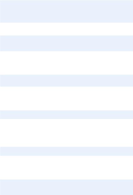
Plotting the Heaviside Function. Since the Heaviside function consists of two flat lines, one may think that we do not need many points along the x axis to describe the curve. Let us try only five points:
x = linspace(-10, 10, 5)
plot(x, Hv(x), axis=[x[0], x[-1], -0.1, 1.1])
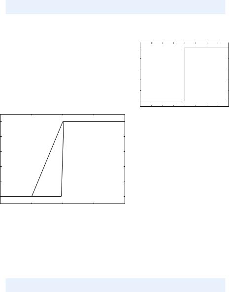
However, so few x points are not able to describe the jump from 0 to 1 at x = 0, as shown by the solid line in Figure 4.10a. Using more points, say 50 between −10 and 10,
x2 = linspace(-10, 10, 50)
plot(x, Hv(x), ’r’, x2, Hv(x2), ’b’,
legend=(’5 points’, ’50 points’), axis=[x[0], x[-1], -0.1, 1.1])
202 |
4 Array Computing and Curve Plotting |
|
|
makes the curve look better, as you can see from the dotted line in Figure 4.10a. However, the step is still not vertical. This time the point x = 0 was not among the coordinates so the step goes from x = −0.2 to x = 0.2. More points will improve the situation. Nevertheless, the best is to draw two flat lines directly: from (−10, 0) to (0, 0), then to (0, 1) and then to (10, 1):
plot([-10, 0, 0, 10], [0, 0, 1, 1],
axis=[x[0], x[-1], -0.1, 1.1])
The result is shown in Figure 4.10b.
1
0.8
0.6
0.4
0.2
0
−4 |
−3 |
−2 |
−1 |
0 |
1 |
2 |
3 |
4 |
|
|
|
|
(b) |
1 |
|
|
|
|
0.8 |
|
|
|
|
0.6 |
|
|
|
|
0.4 |
|
|
|
|
0.2 |
|
|
|
|
0 |
|
|
|
|
−10 |
−5 |
0 |
5 |
10 |
|
|
(a) |
|
|
Fig. 4.10 Plot of the Heaviside function: (a) using equally spaced x points (5 and 50);
(b) using a “double point” at x = 0.
Some will argue that the plot of H(x) should not contain the vertical line from (0, 0) to (0, 1), but only two horizontal lines. To make such a plot, we must draw two distinct curves, one for each horizontal line:
plot([-10,0], [0,0], ’r-’, [0,10], [1,1], ’r-’,
axis=[x[0], x[-1], -0.1, 1.1])
Observe that we must specify the same line style for both lines (curves), otherwise they would by default get di erent color on the screen and di erent line type in a hardcopy. We remark, however, that discontinuous functions like H(x) are often visualized with vertical lines at the jumps, as we do in Figure 4.10b.
4.4 Plotting Di culties |
203 |
|
|
1 |
|
|
|
|
|
|
0.8 |
|
|
|
|
|
|
0.6 |
|
|
|
|
|
|
0.4 |
|
|
|
|
|
|
0.2 |
|
|
|
|
|
|
0 |
|
|
|
|
|
|
−2 |
−1 |
0 |
1 |
2 |
3 |
4 |
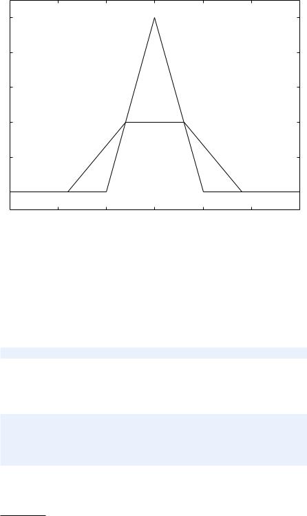
Fig. 4.11 Plot of a “hat” function. The solid line shows the exact function, while the dashed line arises from using inappropriate points along the x axis.
Example: A “Hat” Function. Let us plot the “hat” function N (x), defined by (2.5) on page 89. The corresponding Python implementation N(x) shown right after (2.5) does not work with array arguments x because the boolean expressions, like x < 0, are arrays and they cannot yield a single True or False value for the if tests. The simplest solution is to use vectorize, as explained for the Heaviside function above8:
N_vec = vectorize(N)
A manual rewrite, yielding a faster vectorized function, is more demanding than for the Heaviside function because we now have multiple branches in the if test. One attempt may be9
def Nv(x):
r = where(x < 0, 0.0, x)
r = where(0 <= x < 1, x, r)
r = where(1 <= x < 2, 2-x, r) r = where(x >= 2, 0.0, r) return r
However, the condition like 0 <= x < 1, which is equivalent to 0 <= x and x < 1, does not work because the and operator does not work with array arguments. All operators in Python (+, -, and, or, etc.)
8It is important that N(x) return float and not int values, otherwise the vectorized version will produce int values and hence be incorrect.
9 This is again advanced material.
204 |
4 Array Computing and Curve Plotting |
|
|
are available as pure functions in a module operator (operator.add, operator.sub, operator.and_, operator.or_10, etc.). A working Nv function must apply operator.and_ instead:
def Nv(x):
r = where(x < 0, 0.0, x) import operator
condition = operator.and_(0 <= x, x < 1) r = where(condition, x, r)
condition = operator.and_(1 <= x, x < 2) r = where(condition, 2-x, r)
r = where(x >= 2, 0.0, r) return r
A second, alternative rewrite is to use boolean expressions in indices:
def Nv(x):
r = x.copy() # avoid modifying x in-place r[x < 0.0] = 0.0
condition = operator.and_(0 <= x, x < 1) r[condition] = x[condition]
condition = operator.and_(1 <= x, x < 2) r[condition] = 2-x[condition]
r[x >= 2] = 0.0 return r
Now to the computation of coordinate arrays for the plotting. We may use an explicit loop over all array elements, or the N_vec function, or the Nv function. An approach without thinking about vectorization too much could be
x = linspace(-2, 4, 6)
plot(x, N_vec(x), ’r’, axis=[x[0], x[-1], -0.1, 1.1])
This results in the dashed line in Figure 4.11. What is the problem? The problem lies in the computation of the x vector, which does not contain the points x = 1 and x = 2 where the function makes significant changes. The result is that the “hat” is “flattened”. Making an x vector with all critical points in the function definitions, x = 0, 1, 2, provides the necessary remedy, either
x = linspace(-2, 4, 7)
or the simple
x = [-2, 0, 1, 2, 4]
Any of these x alternatives and a plot(x, N_vec(x)) will result in the solid line in Figure 4.11, which is the correct visualization of the N (x) function.
10Recall that and and or are reserved keywords, see page 10, so a module or program cannot have variables or functions with these names. To circumvent this problem, the convention is to add a trailing underscore to the name.

4.4 Plotting Di culties |
205 |
|
|
4.4.2 Rapidly Varying Functions
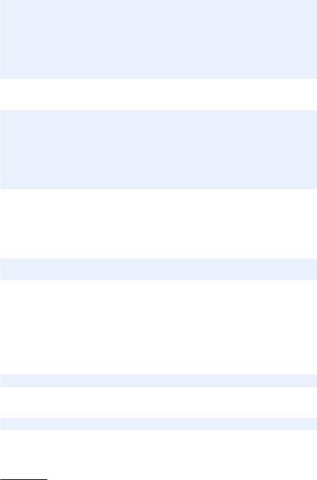
Let us now visualize the function f (x) = sin(1/x), using 10 and 1000 points:
def f(x):
return sin(1.0/x)
x1 = linspace(-1, 1, 10)
x2 = linspace(-1, 1, 1000)
plot(x1, f(x1), label=’%d points’ % len(x)) plot(x2, f(x2), label=’%d points’ % len(x))
The two plots are shown in Figure 4.12. Using only 10 points gives a completely wrong picture of this function, because the function oscillates faster and faster as we approach the origin. With 1000 points we get an impression of these oscillations, but the accuracy of the plot in the vicinity of the origin is still poor. A plot with 100000 points has better accuracy, in principle, but the extermely fast oscillations near the origin just drowns in black ink (you can try it out yourself).
Another problem with the f (x) = sin(1/x) function is that it is easy to define an x vector that contains x = 0, such that we get division by zero. Mathematically, the f (x) function has a singularity at x = 0: it is di cult to define f (0), so one should exclude this point from the function definition and work with a domain x [−1, − ] [ , 1], withchosen small.
The lesson learned from these examples is clear: You must investigate the function to be visualized and make sure that you use an appropriate set of x coordinates along the curve. A relevant first step is to double the number of x coordinates and check if this changes the plot. If not, you probably have an adequate set of x coordinates.
1 |
|
|
|
|
1 |
|
|
|
|
0.8 |
|
|
|
|
0.8 |
|
|
|
|
0.6 |
|
|
|
|
0.6 |
|
|
|
|
0.4 |
|
|
|
|
0.4 |
|
|
|
|
0.2 |
|
|
|
|
0.2 |
|
|
|
|
0 |
|
|
|
|
0 |
|
|
|
|
−0.2 |
|
|
|
|
−0.2 |
|
|
|
|
−0.4 |
|
|
|
|
−0.4 |
|
|
|
|
−0.6 |
|
|
|
|
−0.6 |
|
|
|
|
−0.8 |
|
|
|
|
−0.8 |
|
|
|
|
−1 |
|
|
|
|
−1 |
|
|
|
|
−1 |
−0.5 |
0 |
0.5 |
1 |
−1 |
−0.5 |
0 |
0.5 |
1 |
|
|
(a) |
|
|
|
|
(b) |
|
|
Fig. 4.12 Plot of the function sin(1/x) with (a) 10 points and (b) 1000 points.

206 |
4 Array Computing and Curve Plotting |
|
|
4.4.3 Vectorizing StringFunction Objects
The StringFunction object described in Chapter 3.1.4 does unfortunately not work with array arguments unless we explicitly tell the object to do so. The recipe is very simple. Say f is some StringFunction object. To allow array arguments we must first call f.vectorize(globals()) once:
f = StringFunction(formula) x = linspace(0, 1, 30)
# f(x) will in general not work
from numpy import * f.vectorize(globals())
# now f works with array arguments: values = f(x)
It is important that you import everything from numpy or scitools.std before you call f.vectorize. We suggest to take the f.vectorize call as a magic recipe11.
Even after calling f.vectorize(globals()) a StringFunction object may face problems with vectorization. One example is a piecewise constant function as specified by a string expression ’1 if x > 2 else 0’. One remedy is to use the vectorized version of an if test: ’where(x > 2, 1, 0)’. For an average user of the program this construct is not at all obvious so a more user-friendly solution is to apply vectorize from numpy:
f = vectorize(f) # vectorize a StringFunction f
The line above is therefore the most general (but also the slowest) way of vectorizing a StringFunction object. After that call, f is no more a StringFunction object, but f behaves as a (vectorized) function. The vectorize tool from numpy can be used to allow any Python function taking scalar arguments to also accept array arguments.
To get better speed, one can use vectorize(f) only in the case the formula in f contains an inline if test (e.g., recoginzed by the string ’ else ’ inside the formula). Otherwise, we use f.vectorize. The formula in f is obtained by str(f) so we can test
11Some readers still want to know what the problem is. Inside the StringFunction module we need to have access to mathematical functions for expressions like sin(x)*exp(x) to be evaluated. These mathematical functions are by default taken from the math module and hence they do not work with array arguments. If the user, in the main program, has imported mathematical functions that work with array arguments, these functions are registered in a dictionary returned from globals(). By the f.vectorize call we supply the StringFunction module with the user’s global namespace so that the evaluation of the string expression can make use of mathematical functions for arrays.
4.5 More on Numerical Python Arrays |
207 |
|
|
if ’ else ’ in str(f): f = vectorize(f)
else:
f.vectorize(globals())
4.5 More on Numerical Python Arrays
This section lists some more advanced but useful operations with Numerical Python arrays.
4.5.1 Copying Arrays
Let x be an array. The statement a = x makes a refer to the same array as x. Changing a will then also a ect x:
>>>x = array([1, 2, 3.5])
>>>a = x
>>>a[-1] = 3 # this changes x[-1] too!
>>>x
array([ 1., 2., 3.])
Changing a without changing x requires a to be a copy of x:
>>>a = x.copy()
>>>a[-1] = 9
>>>a
array([ 1., 2., 9.])
>>> x
array([ 1., 2., 3.])
4.5.2 In-Place Arithmetics
Let a and b be two arrays of the same shape. The expression a += b means a = a + b, but this is not the complete story. In the statement a = a + b, the sum a + b is first computed, yielding a new array, and then the name a is bound to this new array. The old array a is lost unless there are other names assigned to this array. In the statement a += b, elements of b are added directly into the elements of a (in memory). There is no hidden intermediate array as in a = a + b. This implies that a += b is more e cient than a = a + b since Python avoids making an extra array. We say that the operators +=, *=, and so on, perform in-place arithmetics in arrays.
Consider the compound array expression