Notes on the electron-phonon interaction Учебное пособие

NOTES ON THE ELECTRON-PHONON INTERACTION

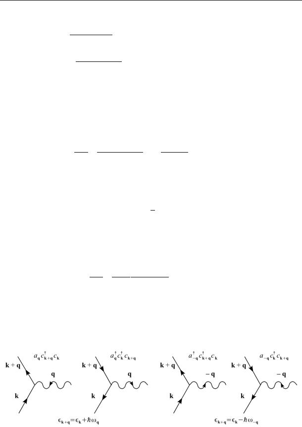
The transition processes described by this Hamiltonian can be represented with the Feynman diagrams in Fig. 1. Above the diagrams we indicate the corresponding term in the Hamiltonian, and below the energy conservation relation.

We shall calculate the electron-phonon-interaction time in two ways. One way to do so is to calculate the probability per unit time that the electron initially in a state k will make a transition to a state k q . Since we are not interested in the final state, we shall be summing over all possible final states, i.e. over all possible values of q. The other way is to solve the Boltzmann kinetic equation in the relaxation time approximation.

Fig. 1. Transition processes described by the Hamiltonian of the electron-phonon interaction

4.1. Electron-phonon-interaction time through the transition probability

Using the Fermi golden rule we write

11

С. А. Рябчун

where the terms in the square brackets correspond to the left and right diagrams, and fk and nq are equilibrium Fermi and Bose distribution functions, respectively. The Bose distribution function only depends on the frequency of the phonon, which, together with the phonon dispersion law (4), ensures that it depends on the absolute value of the phonon wave vector.

Phonon energies are much smaller than electron energies, not least at low temperatures, so we can write

At temperatures well below the Debye temperature the wave vector of a phonon is much smaller than the inverse screening length, so the matrix element in the electron-phonon Hamiltonian simplifies to

Using (33) we can transform the delta-functions as follows:

1

k q q q Fk q F cos cos , (35)

F F

where θ is the angle between the direction of the initial momentum of the electron and the momentum of the phonon. Taking the polar angle along the direction of k and replacing summation over q with integration we rewrite the electron-phonon interaction:

Even at room temperatures the excitation energies of electrons are much smaller that the chemical potential, so the electron-phonon-interaction time is practically independent on the energy of the electron. For the same reason the Fermi distribution function under the integral sign can be well approximated with

12

NOTES ON THE ELECTRON-PHONON INTERACTION

where we have introduced the variable z = ω/T and extended the upper limit of integration to infinity because we work at temperatures much lower than the Debye temperature. With the explicit expression for the Fermi and Bose distribution functions the integrand in the last expression can transformed to yield

The last integral is expressed in terms of the zeta-function:

and we can write the final expression for the electron-phonon-interaction time:

The superscript (1) on the electron-phonon-interaction time is an indication that it has been computed with the first method.

Fig. 2. Diagrams illustrating the processes contributing to the time evolution of the distribution function of the electrons.

13

С. А. Рябчун

4.2. Electron-phonon-interaction time from the kinetic equation

Write down the Boltzmann kinetic equation for the electrons

where f and n are non-equilibrium distribution functions for electrons and phonons, and , is the collision integral. In the relaxation-time approximation the collision integral is written as

where f0 is the equilibrium distribution function of the electrons. Unlike the previous subsection, where we only considered processed given by the terms in the electron-phonon Hamiltonian, we must now also consider the corresponding reverse processes. Indeed, the distribution of electrons in the momentum space changes because electrons come into and leave a particular region of this space. Therefore, instead of the two diagrams of Fig. 1 we now draw four shown in Fig. 2.

We make the following approximations: 1) the collision integral is calculated with the use of the Fermi golden rule; 2) the phonons are in equilibrium.

Thus,

One can check that in thermal equilibrium the collision integral is zero, as it should be, so only departures of the Fermi distributions from their equilibrium values kand k qwill give a non-zero contribution to the relaxation process. We make an approximation k q 0,in which case the Boltzmann equations for different distribution functions are uncoupled, and the collision integral simplifies to

14

NOTES ON THE ELECTRON-PHONON INTERACTION

Using (43) and performing the same manipulations as in sec. 1.4.2 we obtain the electron-phonon-interaction time

where the superscript refers to the method employed for the computation.

15