An Introduction To Statistical Inference And Data Analysis

:5) · 1. If we try P (X = :5) = ² for any real number ² > 0, then a di±culty arises. Because we are assuming that every value in the unit interval is equally likely, it must be that P (X = x) = ² for every x 2 [0; 1]. Consider

which we cannot allow. Hence, we must assign a probability of zero to the outcome x = :5 and, because all outcomes are equally likely, P (X = x) = 0 for every x 2 [0; 1].

Because every x 2 [0; 1] is a possible outcome, our conclusion that P (X = x) = 0 is initially somewhat startling. However, it is a mistake to identify impossibility with zero probability. In Section 2.2, we established that the impossible event (empty set) has probability zero, but we did not say that it is the only such event. To avoid confusion, we now emphasize:

If an event is impossible, then it necessarily has probability zero; however, having probability zero does not necessarily mean that an event is impossible.

If P (X = x) = ² = 0, then the calculation in (4.2) reveals that the event de¯ned by (4.1) has probability zero. Furthermore, there is nothing special about this particular event|the probability of any countable event must be zero! Hence, to obtain positive probabilities, e.g. P (X 2 [0; 1]) = 1, we must consider events whose cardinality is more than countable.

Consider the events [0; :5] and [:5; 1]. Because all outcomes are equally likely, these events must have the same probability, i.e.

P (X 2 [0; :5]) = P (X 2 [:5; 1]) :

Because [0; :5] [ [:5; 1] = [0; 1] and P (X = :5) = 0, we have

Combining these equations, we deduce that each event has probability 1=2. This is an intuitively pleasing conclusion: it says that, if outcomes are equally

What about the pmf of X? In Section 3.1, we de¯ned the pmf of a discrete random variable by f(x) = P (X = x); we then used the pmf to calculate the probabilities of arbitrary events. In the present situation, P (X = x) = 0 for every x, so the pmf is not very useful. Instead of representing the probabilites of individual points, we need to represent the probabilities of intervals.

Consider the function

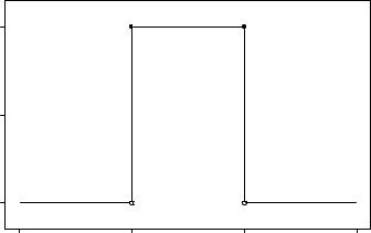
which is plotted in Figure 4.2. Notice that f is constant on X(S) = [0; 1], the set of equally likely possible values, and vanishes elsewhere. If 0 · a · b · 1, then the area under the graph of f between a and b is the area of a rectangle with sides b ¡a (horizontal direction) and 1 (vertical direction). Hence, the area in question is

(b ¡ a) ¢ 1 = b ¡ a = P (X 2 [a; b]);

so that the probabilities of intervals can be determined from f. In the next section, we will base our de¯nition of continuous random variables on this observation.

4.2Basic Concepts

Consider the graph of a function f : < ! <, as depicted in Figure 4.3. Our interest is in the area of the shaded region. This region is bounded by the graph of f, the horizontal axis, and vertical lines at the speci¯ed endpoints

a and b. We denote this area by Area[a;b](f). Our intent is to identify such areas with the probabilities that random variables assume certain values.

For a very few functions, such as the one de¯ned in (4.3), it is possible to determine Area[a;b](f) by elementary geometric calculations. For most functions, some knowledge of calculus is required to determine Area[a;b](f). Because we assume no previous knowledge of calculus, we will not be concerned with such calculations. Nevertheless, for the bene¯t of those readers who know some calculus, we ¯nd it helpful to borrow some notation and

f(x)

x

Figure 4.3: A Continuous Probability Density Function

Readers who have no knowledge of calculus should interpret (4.4) as a definition of its right-hand side, which is pronounced \the integral of f from a to b". Readers who are familiar with the Riemann (or Lebesgue) integral should interpret this notation in its conventional sense.

We now introduce an alternative to the probability mass function.

De¯nition 4.1 A probability density function (pdf) is a function f : < ! < such that

1.f(x) ¸ 0 for every x 2 <.

2.Area(¡1;1](f) = R¡11 f(x)dx = 1.

Notice that the de¯nition of a pdf is analogous to the de¯nition of a pmf. Each is nonnegative and assigns unit probability to the set of possible values. The only di®erence is that summation in the de¯nition of a pmf is replaced with integration in the case of a pdf.

De¯nition 4.1 was made without reference to a random variable|we now use it to de¯ne a new class of random variables.

De¯nition 4.2 A random variable X is continuous if there exists a probability density function f such that

Z b

P (X 2 [a; b]) = f(x)dx:

a

It is immediately apparent from this de¯nition that the cdf of a continuous random variable X is

¡1

Equation (4.5) should be compared to equation (3.1). In both cases, the value of the cdf at y is represented as the accumulation of values of the pmf/pdf at x · y. The di®erence lies in the nature of the accumulating process: summation for the discrete case (pmf), integration for the continuous case (pdf).

Remark for Calculus Students: By applying the Fundamental Theorem of Caluclus to (4.5), we deduce that the pdf of a continuous random variable is the derivative of its cdf:

Remark on Notation: It may strike the reader as curious that we have used f to denote both the pmf of a discrete random variable and the pdf of a continuous random variable. However, as our discussion of their relation to the cdf is intended to suggest, they play analogous roles. In advanced, measure-theoretic courses on probability, one learns that our pmf and pdf are actually two special cases of one general construction.

Likewise, the concept of expectation for continuous random variables is analogous to the concept of expectation for discrete random variables. Because P (X = x) = 0 if X is a continuous random variable, the notion of a probability-weighted average is not very useful in the continuous setting. However, if X is a discrete random variable, then P (X = x) = f(x) and a probability-weighted average is identical to a pmf-weighted average. In

Example 1 What is the probability that a battery-powered wristwatch will stop with its minute hand positioned between 10 and 20 minutes past the hour?

To answer this question, let X denote the number of minutes past the hour to which the minute hand points when the watch stops. Then the possible values of X are X(S) = [0; 60) and it is reasonable to assume that each value is equally likely. We must compute P (X 2 (10; 20)). Because these values occupy one sixth of the possible values, it should be obvious that the answer is going to be 1=6.

To obtain the answer using the formal methods of probability, we require a generalization of the Uniform[0; 1] distribution that we studied in Section 4.1. The pdf that describes the notion of equally likely values in the interval

To check that f is really a pdf, observe that f(x) ¸ 0 for every x 2 < and

that

1 Area[0;60)(f) = (60 ¡ 0)60 = 1:

Notice the analogy between the pdfs (4.6) and (4.3). The present pdf de¯nes the continuous uniform distribution on the interval [0; 60); thus, we describe the present situation by writing X » Uniform[0; 60). To calculate the spec- i¯ed probability, we must determine the area of the shaded region in Figure 4.4, i.e.

Example 2 Consider two battery-powered watches. Let X1 denote the number of minutes past the hour at which the ¯rst watch stops and let X2 denote the number of minutes past the hour at which the second watch stops. What is the probability that the larger of X1 and X2 will be between 30 and

50?

Here we have two independent random variables, each distributed as Uniform[0; 60), and a third random variable,

Y = max(X1; X2):