An Introduction To Statistical Inference And Data Analysis

Example 4 Consider the disjoint events depicted in Figure 2.7 and suppose that P (A) > 0 and P (B) > 0. Are A and B independent? Many students instinctively answer that they are, but independence is very different from mutual exclusivity. In fact, if A occurs then B does not (and vice versa), so Figure 2.7 is actually a fairly extreme example of dependent events. This can also be deduced from De¯nition 2.2: P (A) ¢P (B) > 0, but

P (A \ B) = P (;) = 0

so A and B are not independent.

Example 5 For each of the following, explain why the events A and B are or are not independent.

(a)P (A) = :4, P (B) = :5, P ([A [ B]c) = :3. It follows that

P (A [ B) = 1 ¡ P ([A [ B]c) = 1 ¡ :3 = :7

and, because P (A [ B) = P (A) + P (B) ¡ P (A \ B), that

P (A \ B) = P (A) + P (B) ¡ P (A [ B) = :4 + :5 ¡ :7 = :2:

Then, since

P (A) ¢ P (B) = :5 ¢ :4 = :2 = P (A \ B);

it follows that A and B are independent events.

(b)P (A \ Bc) = :3, P (Ac \ B) = :2, P (Ac \ Bc) = :1. Refer to the Venn diagram in Figure 2.8 to see that

P (A) ¢ P (B) = :7 ¢ :6 = :42 6= :40 = P (A \ B)

and hence that A and B are dependent events.

Thus far we have veri¯ed that two events are independent by verifying that the multiplication rule for independence holds. In applications, however, we usually reason somewhat di®erently. Using our intuitive notion of independence, we appeal to common sense, our knowledge of science, etc., to decide if independence is a property that we wish to incorporate into our mathematical model of the experiment in question. If it is, then we assume that two events are independent and the multiplication rule for independence becomes available to us for use as a computational formula.

Figure 2.8: Venn Diagram for Example 5

Example 6 Consider an experiment in which a typical penny is ¯rst tossed, then spun. Let A denote the event that the toss results in Heads and let B denote the event that the spin results in Heads. What is the probability of observing two Heads?

For a typical penny, P (A) = :5 and P (B) = :3. Common sense tells us that the occurrence of either event is una®ected by the occurrence of the other. (Time is not reversible, so obviously the occurrence of A is not a®ected by the occurrence of B. One might argue that tossing the penny so that A occurs results in wear that is slightly di®erent than the wear that results if Ac occurs, thereby slightly a®ecting the subsequent probability that B occurs. However, this argument strikes most students as completely preposterous. Even if it has a modicum of validity, the e®ect is undoubtedly so slight that we can safely neglect it in constructing our mathematical model of the experiment.) Therefore, we assume that A and B are independent and calculate that

P (A \ B) = P (A) ¢ P (B) = :5 ¢ :3 = :15:

Example 7 For each of the following, explain why the events A and B are or are not independent.

(a)Consider the population of William & Mary undergraduate students, from which one student is selected at random. Let A denote the event that the student is female and let B denote the event that the student is concentrating in education.

I'm told that P (A) is roughly 60 percent, while it appears to me that P (AjB) exceeds 90 percent. Whatever the exact probabilities, it is evident that the probability that a random education concentrator is female is considerably greater than the probability that a random student is female. Hence, A and B are dependent events.

(b)Consider the population of registered voters, from which one voter is selected at random. Let A denote the event that the voter belongs to a country club and let B denote the event that the voter is a Republican.

It is generally conceded that one ¯nds a greater proportion of Republicans among the wealthy than in the general population. Since one tends to ¯nd a greater proportion of wealthy persons at country clubs than in the general population, it follows that the probability that a random country club member is a Republican is greater than the probability that a randomly selected voter is a Republican. Hence, A and B are dependent events.3

Before progressing further, we ask what it should mean for A, B, and C to be three mutually independent events. Certainly each pair should comprise two independent events, but we would also like to write

P (A \ B \ C) = P (A) ¢ P (B) ¢ P (C):

It turns out that this equation cannot be deduced from the pairwise independence of A, B, and C, so we have to include it in our de¯nition of mutual independence. Similar equations must be included when de¯ning the mutual independence of more than three events. Here is a general de¯nition:

De¯nition 2.3 Let fA®g be an arbitrary collection of events. These events are mutually independent if and only if, for every ¯nite choice of events

3This phenomenon may seem obvious, but it was overlooked by the respected Literary Digest poll. Their embarrassingly awful prediction of the 1936 presidential election resulted in the previously popular magazine going out of business. George Gallup's relatively accurate prediction of the outcome (and his uncannily accurate prediction of what the Literary Digest poll would predict) revolutionized polling practices.

A®1 ; : : : ; A®k ,

P (A®1 \¢¢¢\ A®k ) = P (A®1 ) ¢¢¢P (A®k ) :

Example 8 In the preliminary hearing for the criminal trial of O.J. Simpson, the prosecution presented conventional blood-typing evidence that blood found at the murder scene possessed three characteristics also possessed by Simpson's blood. The prosecution also presented estimates of the prevalence of each characteristic in the general population, i.e. of the probabilities that a person selected at random from the general population would possess these characteristics. Then, to obtain the estimated probability that a randomly selected person would possess all three characteristics, the prosecution multiplied the three individual probabilities, resulting in an estimate of :005.

In response to this evidence, defense counsel Gerald Uehlman objected that the prosecution had not established that the three events in question were independent and therefore had not justi¯ed their use of the multiplication rule. The prosecution responded that it was standard practice to multiply such probabilities and Judge Kennedy-Powell admitted the :005 estimate on that basis. No attempt was made to assess whether or not the standard practice was proper; it was inferred from the fact that the practice was standard that it must be proper. In this example, science and law diverge. From a scienti¯c perspective, Gerald Uehlman was absolutely correct in maintaining that an assumption of independence must be justi¯ed.

2.5Random Variables

Informally, a random variable is a rule for assigning real numbers to experimental outcomes. By convention, random variables are usually denoted by upper case Roman letters near the end of the alphabet, e.g. X, Y , Z.

Example 1 A coin is tossed once and Heads (H) or Tails (T) is observed.

The sample space for this experiment is S = fH; Tg. For reasons that will become apparent, it is often convenient to assign the real number 1 to Heads and the real number 0 to Tails. This assignment, which we denote

by the random variable X, can be depicted as follows:

In functional notation, X : S ! < and the rule of assignment is de¯ned by

X(H) = 1;

X(T) = 0:

Example 2 A coin is tossed twice and the number of Heads is counted.

The sample space for this experiment is S = fHH; HT; TH; TTg. We want to assign the real number 2 to the outcome HH, the real number 1 to the outcomes HT and TH, and the real number 0 to the outcome TT. Several representations of this assignment are possible:

(a)Direct assignment, which we denote by the random variable Y , can be depicted as follows:

In functional notation, Y : S ! < and the rule of assignment is de¯ned by

Y (HH) = 2;

Y (HT) = Y (TH) = 1;

Y (TT) = 0:

(b)Instead of directly assigning the counts, we might take the intermediate step of assigning an ordered pair of numbers to each outcome. As in Example 1, we assign 1 to each occurence of Heads and 0 to each occurence of Tails. We denote this assignment by X : S ! <2. In this context, X = (X1; X2) is called a random vector. Each component of the random vector X is a random variable.

Next, we de¯ne a function g : <2 ! < by

g(x1; x2) = x1 + x2:

The composition g(X) is equivalent to the random variable Y , as revealed by the following depiction:

(c)The preceding representation suggests de¯ning two random variables, X1 and X2, as in the following depiction:

As in the preceding representation, the random variable X1 counts the number of Heads observed on the ¯rst toss and the random variable X2 counts the number of Heads observed on the second toss. The sum of these random variables, X1 +X2, is evidently equivalent to the random variable Y .

The primary reason that we construct a random variable, X, is to replace the probability space that is naturally suggested by the experiment in question with a familiar probability space in which the possible outcomes are real numbers. Thus, we replace the original sample space, S, with the familiar number line, <. To complete the transference, we must decide which subsets of < will be designated as events and we must specify how the probabilities of these events are to be calculated.

It is an interesting fact that it is impossible to construct a probability space in which the set of outcomes is < and every subset of < is an event. For this reason, we de¯ne the collection of events to be the smallest collection of subsets that satis¯es the assumptions of the Kolmogorov probability model and that contains every interval of the form (¡1; y]. This collection is called the Borel sets and it is a very large collection of subsets of <. In particular, it contains every interval of real numbers and every set that can be constructed by applying a countable number of set operations (union, intersection, complementation) to intervals. Most students will never see a set that is not a Borel set!

Finally, we must de¯ne a probability measure that assigns probabilities to Borel sets. Of course, we want to do so in a way that preserves the probability structure of the experiment in question. The only way to do so is to de¯ne the probability of each Borel set B to be the probability of the set of outcomes to which X assigns a value in B. This set of outcomes is denoted by

X¡1(B) = fs 2 S : X(s) 2 Bg

and is depicted in Figure 2.9.

How do we know that the set of outcomes to which X assigns a value in B is an event and therefore has a probability? We don't, so we guarantee

Figure 2.9: The Inverse Image of a Borel Set

that it is by including this requirement in our formal de¯nition of random variable.

De¯nition 2.4 A function X : S ! < is a random variable if and only if

P (fs 2 S : X(s) · yg)

exists for all choices of y 2 <.

We will denote the probability measure induced by the random variable X by PX . The following equation de¯nes various representations of PX :

³´

PX ((¡1; y]) = P X¡1 ((¡1; y])

=P (fs 2 S : X(s) 2 (¡1; y]g)

=P (¡1 < X · y)

=P (X · y)

A probability measure on the Borel sets is called a probability distribution and PX is called the distribution of the random variable X. A hallmark feature of probability theory is that we study the distributions of random variables rather than arbitrary probability measures. One important reason

for this emphasis is that many di®erent experiments may result in identical distributions. For example, the random variable in Example 1 might have the same distribution as a random variable that assigns 1 to male newborns and 0 to female newborns.

Cumulative Distribution Functions Our construction of the probability measure induced by a random variable suggests that the following function will be useful in describing the properties of random variables.

De¯nition 2.5 The cumulative distribution function (cdf) of a random variable X is the function F : < ! < de¯ned by

F (y) = P (X · y):

Example 1 (continued) We consider two probability structures that might obtain in the case of a typical penny.

(a)A typical penny is tossed.

In this experiment, P (H) = P (T) = :5, and the following values of the cdf are easily determined:

{If y < 0, e.g. y = ¡:3018, then

F (y) = P (X · y) = P (;) = 0:

{F (0) = P (X · 0) = P (fTg) = :5.

{If y 2 (0; 1), e.g. y = :9365, then

F (y) = P (X · y) = P (fTg) = :5:

{F (1) = P (X · 1) = P (fT; Hg) = 1.

{If y > 1, e.g. y = 1:5248, then

F (y) = P (X · y) = P (fT; Hg) = 1:

The entire cdf is plotted in Figure 2.10.

(b)A typical penny is spun.

In this experiment, P (H) = :3, P (T) = :7, and the following values of the cdf are easily determined:

Figure 2.10: Cumulative Distribution Function for Tossing a Typical Penny

{ If y < 0, e.g. y = ¡:5485, then

F (y) = P (X · y) = P (;) = 0:

{F (0) = P (X · 0) = P (fTg) = :7.

{If y 2 (0; 1), e.g. y = :0685, then

F (y) = P (X · y) = P (fTg) = :7:

{F (1) = P (X · 1) = P (fT; Hg) = 1.

{If y > 1, e.g. y = 1:4789, then

F (y) = P (X · y) = P (fT; Hg) = 1:

The entire cdf is plotted in Figure 2.11.

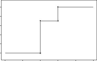
Example 2 (continued) Suppose that the coin is fair, so that each of the four possible outcomes in S is equally likely, i.e. has probability :25. Then the following values of the cdf are easily determined:

Figure 2.11: Cumulative Distribution Function for Spinning a Typical Penny

² If y < 0, e.g. y = ¡:5615, then

F (y) = P (X · y) = P (;) = 0:

²F (0) = P (X · 0) = P (fTTg) = :25.

²If y 2 (0; 1), e.g. y = :3074, then

F (y) = P (X · y) = P (fTTg) = :25:

²F (1) = P (X · 1) = P (fTT; HT; THg) = :75.

²If y 2 (1; 2), e.g. y = 1:4629, then

F (y) = P (X · y) = P (fTT; HT; THg) = :75:

²F (2) = P (X · 2) = P (fTT; HT; TH; HHg) = 1.

²If y > 2, e.g. y = 2:1252, then

F (y) = P (X · y) = P (fTT; HT; TH; HHg) = 1:

The entire cdf is plotted in Figure 2.12.