An Introduction To Statistical Inference And Data Analysis

F= Y1=º1: Y2=º2

Because Yi ¸ 0, the set of possible values of F is F (S) = [0; 1). We are interested in the distribution of F .

De¯nition 4.8 The distribution of F is called an F distribution with º1 and º2 degrees of freedom. We will denote this distribution by F (º1; º2). It is customary to call º1 the \numerator" degrees of freedom and º2 the

\denominator" degrees of freedom.

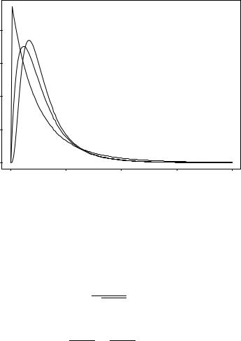
Figure 4.10 displays the pdfs of several F distributions.

There is an important relation between t and F distributions. To anticipate it, suppose that Z » Normal(0; 1) and Y2 » Â2(º2) are independent

More generally,

Theorem 4.5 If T » t(º), then T 2 » F (1; º).

The S-Plus function pf returns values of the cdf of any speci¯ed F distribution. For example, if F » F (2; 27), then P (F > 2:5) is

> 1-pf(2.5,df1=2,df2=27) [1] 0.1008988

106 CHAPTER 5. QUANTIFYING POPULATION ATTRIBUTES

Where is the \middle" of a normal distribution?

It is quite evident from Figure 4.7 that there is only one plausible answer to this question: if X » Normal(¹; ¾2), then the \middle" of the distribution of X is ¹.

Let f denote the pdf of X. To understand why ¹ is the only plausible middle of f, recall a property of f that we noted in Section 4.4: for any x, f(¹+ x) = f(¹¡x). This property states that f is symmetric about ¹. It is the property of symmetry that restricts the plausible locations of \middle" to the central value ¹.

To generalize the above example of a measure of centrality, we introduce an important qualitative property that a population may or may not possess:

De¯nition 5.1 Let X be a continuous random variable with probability density function f. If there exists a value µ 2 < such that

f(µ + x) = f(µ ¡ x)

for every x 2 <, then X is a symmetric random variable and µ is its center of symmetry.

We have already noted that X » Normal(¹; ¾2) has center of symmetry ¹. Another example of symmetry is illustrated in Figure 5.1: X » Uniform[a; b] has center of symmetry (a + b)=2.

For symmetric random variables, the center of symmetry is the only plausible measure of centrality|of where the \middle" of the distribution is located. Symmetry will play an important role in our study of statistical inference. Our primary concern will be with continuous random variables, but the concept of symmetry can be used with other random variables as well. Here is a general de¯nition:

De¯nition 5.2 Let X be a random variable. If there exists a value µ 2 < such that the random variables X ¡µ and µ ¡X have the same distribution, then X is a symmetric random variable and µ is its center of symmetry.

Suppose that we attempt to compute the expected value of a symmetric random variable X with center of symmetry µ. Thinking of the expected value as a weighted average, we see that each µ+x will be weighted precisely as much as the corresponding µ ¡ x. Thus, if the expect value exists (there are a few pathological random variables for which the expected value is unde¯ned), then it must equal the center of symmetry, i.e. EX = µ. Of course, we have already seen that this is the case for X » Normal(¹; ¾2) and for X » Uniform[a; b].

f(x)

x

Figure 5.1: X » Uniform[a; b] has center of symmetry (a + b)=2.

5.2Quantiles

In this section we introduce population quantities that can be used for a variety of purposes. As in Section 5.1, these quantities are most easily understood in the case of continuous random variables:

De¯nition 5.3 Let X be a continuous random variable and let ® 2 (0; 1). If q = q(X; ®) is such that P (X < q) = ® and P (X > q) = 1 ¡ ®, then q is called an ® quantile of X.

If we express the probabilities in De¯nition 5.3 as percentages, then we see that q is the 100® percentile of the distribution of X.

Example 1 Suppose that X » Uniform[a; b] has pdf f, depicted in Figure 5.2. Then q is the value in (a; b) for which

1

® = P (X < q) = Area[a;q](f) = (q ¡ a) ¢ b ¡ a;

i.e. q = a + ®(b ¡ a). This expression is easily interpreted: to the lower endpoint a, add 100®% of the distance b ¡ a to obtain the 100® percentile.

108 CHAPTER 5. QUANTIFYING POPULATION ATTRIBUTES

f(x)

x

Figure 5.2: A quantile of a Uniform distribution.

Example 2 Suppose that X has pdf

()

depicted in Figure 5.3. Then q is the value in (0; 2) for which

i.e. q = 2®.

Example 3 Suppose that X » Normal(0; 1) has cdf F . Then q is the value in (¡1; 1) for which ® = P (X < q) = F (q), i.e. q = F ¡1(®). Unlike the previous examples, we cannot compute q by elementary calculations. Fortunately, the S-Plus function qnorm computes quantiles of normal distributions. For example, we compute the ® = 0:95 quantile of X as follows:

> qnorm(.95) [1] 1.644854

Figure 5.3: A quantile of another distribution.

Example 4 Suppose that X has pdf

depicted in Figure 5.4. Notice that P (X 2 [0; 1]) = 0:5 and P (X 2 [2; 3]) = 0:5. If ® 2 (0; 0:5), then we can use the same reasoning that we employed in Example 1 to deduce that q = 2®. Similarly, if ® 2 (0:5; 1), then q = 2+2(®¡0:5) = 2®+1. However, if ® = 0:5, then we encounter an ambiguity: the equalities P (X < q) = 0:5 and P (X > q) = 0:5 hold for any q 2 [1; 2]. Accordingly, any q 2 [1; 2] is an ® = 0:5 quantile of X. Thus, quantiles are not always unique.

To avoid confusion when a quantile are not unique, it is nice to have a convention for selecting one of the possible quantile values. In the case that ® = 0:5, there is a universal convention:

De¯nition 5.4 The midpoint of the interval of all values of the ® = 0:5 quantile is called the population median.