An Introduction To Statistical Inference And Data Analysis

modate any speci¯ed signi¯cance level. As a practical matter, however, ® must be speci¯ed and we now ask how to do so.

In the penny-spinning example, Robin is making a personal decision and is free to choose ® as she pleases. In the termite example, the researchers were in°uenced by decades of scienti¯c convention. In 1925, in his extremely in°uential Statistical Methods for Research Workers, Ronald Fisher3 suggested that ® = :05 and ® = :01 are often appropriate signi¯cance levels. These suggestions were intended as practical guidelines, but they have become enshrined (especially ® = :05) in the minds of many scientists as a sort of Delphic determination of whether or not a hypothesized theory is true. While some degree of conformity is desirable (it inhibits a researcher from choosing|after the fact|a signi¯cance level that will permit rejecting the null hypothesis in favor of the alternative in which s/he may be invested), many statisticians are disturbed by the scienti¯c community's slavish devotion to a single standard and by its often uncritical interpretation of the resulting conclusions.4

The imposition of an arbitrary standard like ® = :05 is possible because of the precision with which mathematics allows hypothesis testing to be formulated. Applying this precision to legal paradigms reveals the issues with great clarity, but is of little practical value when specifying a signi¯- cance level, i.e. when trying to de¯ne the meaning of \beyond a reasonable doubt." Nevertheless, legal scholars have endeavored for centuries to position \beyond a reasonable doubt" along the in¯nite gradations of assent that correspond to the continuum [0; 1] from which ® is selected. The phrase \beyond a reasonable doubt" is still often connected to the archaic phrase \to a moral certainty." This connection survived because moral certainty was actually a signi¯cance level, intended to invoke an enormous body of scholarly writings and specify a level of assent:

Throughout this development two ideas to be conveyed to the jury have been central. The ¯rst idea is that there are two realms of human knowledge. In one it is possible to obtain the absolute

3Sir Ronald Fisher is properly regarded as the single most important ¯gure in the history of statistics. It should be noted that he did not subscribe to all of the particulars of the Neyman-Pearson formulation of hypothesis testing. His fundamental objection to it, that it may not be possible to fully specify the alternative hypothesis, does not impact our development, since we are concerned with situations in which both hypotheses are fully speci¯ed.

4See, for example, J. Cohen (1994). The world is round (p < :05). American Psychologist, 49:997{1003.

certainty of mathematical demonstration, as when we say that the square of the hypotenuse is equal to the sum of the squares of the other two sides of a right triangle. In the other, which is the empirical realm of events, absolute certainty of this kind is not possible. The second idea is that, in this realm of events, just because absolute certainty is not possible, we ought not to treat everything as merely a guess or a matter of opinion. Instead, in this realm there are levels of certainty, and we reach higher levels of certainty as the quantity and quality of the evidence available to us increase. The highest level of certainty in this empirical realm in which no absolute certainty is possible is what traditionally was called \moral certainty," a certainty which there was no reason to doubt.5

Although it is rarely (if ever) possible to quantify a juror's level of assent, those comfortable with statistical hypothesis testing may be inclined to wonder what values of ® correspond to conventional interpretations of reasonable doubt. If a juror believes that there is a 5 percent probability that chance alone could have produced the circumstantial evidence presented against a defendant accused of pre-meditated murder, is the juror's level of assent beyond a reasonable doubt and to a moral certainty? We hope not. We may be willing to tolerate a 5 percent probability of a Type I error when studying termite foraging behavior, but the analogous prospect of a 5 percent probability of wrongly convicting a factually innocent defendant is abhorrent.6

In fact, little is known about how anyone in the legal system quanti¯es reasonable doubt. Mary Gray cites a 1962 Swedish case in which a judge trying an overtime parking case explicitly ruled that a signi¯cance probability of 1=20; 736 was beyond reasonable doubt but that a signi¯cance probability of 1=144 was not.7 In contrast, Alan Dershowitz relates a provocative classroom exercise in which his students preferred to acquit in one scenario

5Barbara J. Shapiro (1991). \Beyond Reasonable Doubt" and \Probable Cause": Historical Perspectives on the Anglo-American Law of Evidence, University of California Press, Berkeley, p. 41.

6This discrepancy illustrates that the consequences of committing a Type I error in- °uence the choice of a signi¯cance level. The consequences of Jones and Trosset wrongly concluding that termite species compete are not commensurate with the consequences of wrongly imprisoning a factually innocent citizen.

7M.W. Gray (1983). Statistics and the law. Mathematics Magazine, 56:67{81. As a graduate of Rice University, I cannot resist quoting another of Gray's examples of statistics- as-evidence: \In another case, that of millionaire W. M. Rice, the signature on his will

de¯nes an event that may or may not occur each time the experiment is performed. Speci¯cally, (8.3) is the event that the sample mean assumes a value at least as far from the hypothesized mean as the researcher observed.

4.The signi¯cance probability, P , is the probability that (8.3) occurs.

The notation P¹0 reminds us that we are interested in the probability that this event occurs under the assumption that the null hypothesis is true, i.e. under the assumption that ¹ = ¹0.

Having formulated an appropriate signi¯cance probability for testing H0 : ¹ = ¹0 versus H1 : ¹ 6= ¹0, our second challenge is to ¯nd a way to compute P . We remind the reader that we have assumed that n is large.

Case 1: The population variance is known or speci¯ed by the null hypothesis.

We de¯ne two new quantities, the random variable

¹ ¡

Zn = X¾=n pn¹0

and the real number

x¹n ¡ ¹0 z = ¾=pn :

Under the null hypothesis H0 : ¹ = ¹0, Zn»Normal(0; 1) by the Central Limit Theorem; hence,

= 2©(¡jzj);

which can be computed by the S-Plus command

> 2*pnorm(-abs(z))

or by consulting a table. An illustration of the normal probability of interest is sketched in Figure 8.1.

Example 1 To test H0 : ¹ = :5 versus H1 : ¹ 6= :5 at signi¯cance level ® = :05, we perform n = 2500 trials and observe 1200 successes. Should H0 be rejected?

The observed proportion of successes is x¹n = 1200=2500 = :48, so the value of the test statistic is

8.4. TESTING HYPOTHESES ABOUT A POPULATION MEAN 165

and the signi¯cance probability is

: :

P = 2©(¡2) = :0456 < :05 = ®:

Because P · ®, we reject H0.

Case 2: The population variance is unknown.

Because ¾2 is unknown, we must estimate it from the sample. We will use the estimator introduced in Section 8.2,

Theorem 6.3 that

lim P (Tn · z) = ©(z):

n!1

Just as we could use a normal approximation to compute probabilities involving Zn, so can we use a normal approximation to compute probabilities involving Tn. The fact that we must estimate ¾2 slightly degrades the quality of the approximation; however, because n is large, we should observe an accurate estimate of ¾2 and the approximation should not su®er much. Accordingly, we proceed as in Case 1, using

t = x¹n ¡p¹0 sn= n

instead of z.

Example 2 To test H0 : ¹ = 1 versus H1 : ¹ 6= 1 at signi¯cance level ® = :05, we collect n = 2500 observations, observing x¹n = 1:1 and sn = 2. Should H0 be rejected?

The value of the test statistic is

t = 1:1 ¡ 1:0 = 2:5 2=50

and the signi¯cance probability is

: :

P = 2©(¡2:5) = :0124 < :05 = ®:

Because P · ®, we reject H0.

8.4. TESTING HYPOTHESES ABOUT A POPULATION MEAN 167

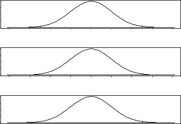
Example 2 (continued) Applying the above reasoning to t = 2:5, we obtain the signi¯cance probabilities sketched in Figure 8.2. Notice that Pb = Pa=2 and that Pb + Pc = 1. The probability Pb is quite small, so we reject H0 : ¹ · 1. This makes sense, because we observed x¹n = 1:1 > 1:0 = ¹0. It is therefore obvious that the sample contains some evidence that ¹ > 1 and the statistical test reveals that the strength of this evidence is fairly compelling.

Figure 8.2: Signi¯cance Probabilities for Example 2

In contrast, the probability of Pc is quite large and so we decline to reject H0 : ¹ ¸ 1. This also makes sense, because the sample contains no evidence that ¹ < 1. In such instances, performing a statistical test only con¯rms that which is transparent from comparing the sample and hypothesized means.

Example 3 A group of concerned parents wants speed humps installed in front of a local elementary school, but the city tra±c o±ce is reluctant to allocate funds for this purpose. Both parties agree that humps should be installed if the average speed of all motorists who pass the school while it is in session exceeds the posted speed limit of 15 miles per hour (mph). Let ¹ denote the average speed of the motorists in question. A random sample of

n = 150 of these motorists was observed to have a sample mean of x¹ = 15:3 mph with a sample standard deviation of s = 2:5 mph.

(a)State null and alternative hypotheses that are appropriate from the parents' perspective.

(b)State null and alternative hypotheses that are appropriate from the city tra±c o±ce's perspective.

(c)Compute the value of an appropriate test statistic.

(d)Adopting the parents' perspective and assuming that they are willing to risk a 1% chance of committing a Type I error, what action should be taken? Why?

(e)Adopting the city tra±c o±ce's perspective and assuming that they are willing to risk a 10% chance of committing a Type I error, what action should be taken? Why?

Solution

(a)Absent compelling evidence, the parents want to install the speed humps that they believe will protect their children. Thus, the null hypothesis to which the parents will default is H0 : ¹ ¸ 15. The parents require compelling evidence that speed humps are unnecessary, so their alternative hypothesis is H1 : ¹ < 15.

(b)Absent compelling evidence, the city tra±c o±ce wants to avoid spending taxpayer dollars that might fund other public works. Thus, the null hypothesis to which the tra±c o±ce will default is H0 : ¹ · 15. The tra±c o±ce requires compelling evidence that speed humps are necessary, so its alternative hypothesis is H1 : ¹ > 15.

(c)Because the population variance is unknown, the appropriate test

(d)We would reject the null hypothesis in (a) if x¹ is su±ciently smaller

than ¹0 = 15. Since x¹ = 15:3 > 15, there is no evidence against H0 : ¹ ¸ 15. The null hypothesis is retained and speed humps are installed.

8.4. TESTING HYPOTHESES ABOUT A POPULATION MEAN 169

(e)We would reject the null hypothesis in (b) if x¹ is su±ciently larger than ¹0 = 15, i.e. for su±ciently large positive values of t. Hence, the signi¯cance probability is

Because P · ®, the tra±c o±ce should reject H0 : ¹ · 15 and install speed humps.

Statistical Signi¯cance and Material Signi¯cance

The signi¯cance probability is the probability that a coincidence at least as extraordinary as the phenomenon observed can be produced by chance. The smaller the signi¯cance probability, the more con¯dently we reject the null hypothesis. However, it is one thing to be convinced that the null hypothesis is incorrect|it is something else to assert that the true state of nature is very di®erent from the state(s) speci¯ed by the null hypothesis.

Example 4 A government agency requires prospective advertisers to provide statistical evidence that documents their claims. In order to claim that a gasoline additive increases mileage, an advertiser must fund an independent study in which n vehicles are tested to see how far they can drive, ¯rst without and then with the additive. Let Xi denote the increase in miles per gallon (mpg with the additive minus mpg without the additive) observed for vehicle i and let ¹ = EXi. The null hypothesis H0 : ¹ · 1 is tested against the alternative hypothesis H1 : ¹ > 1 and advertising is authorized if H0 is rejected at a signi¯cance level of ® = :05.

Consider the experiences of two prospective advertisers:

1.A large corporation manufactures an additive that increases mileage by an average of ¹ = 1:01 miles per gallon. The corporation funds a large study of n = 900 vehicles in which x¹ = 1:01 and s = 0:1 are observed. This results in a test statistic of

P = P (Tn ¸ t) = P (Z ¸ 3) = 1 ¡ ©(3) = 0:00135 < 0:05 = ®:

The null hypothesis is decisively rejected and advertising is authorized.