

Algebraic equation system
The magnetization of each element is considered constant. More complex approximation schemes are not used
To form a system of equations the method is collocations is used
M lk |
|
|
|
|
C kj M iV |
j |
H k |
|
|
|
|
||||||
l |
1 |
|
lj |
j |
cl |
|||
|
j,i |
|
|
|
|
|||
11
Finite element method
12
Main steps
0. Problem formulation – problem domain, equation, boundary conditions, material properties
1.Discretization of the problem domain.
2.Approximation of the unknown function.
3.Approximation of the solved equation and the boundary conditions.
4.Solution of the algebraic equation system (generally – nonlinear).
5.Post-processing.
13
Discretization.
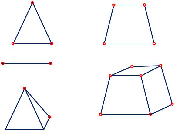
The element type choice.
2D
problem:
1D
problem:
3D
problem:

 Octahedron (8 nodes) Tetrahedron (4 nodes) 14

Discretization. Examples of the mesh.
15

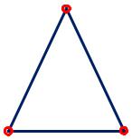
Linear approximation
‘1’
|
U (x, y) a bx cy |
|
‘2’ |
‘3’ Nodal potentials: |
U1, U2 , U3 |
The number of free parameters is the same!
In principle we can express coefficients a, b, c in terms of the nodal potentials U1, U2 U3
16
Finite functions
|
‘1’ |
i (x, y) ai bi x ci y |
i 1,2,3 |
‘2’ |
|
The main properties: 1 (x1, y1 ) 1 |
|
‘3’ |
1(x2 , y2 ) 0 |
|
1 (x3 , y3 ) 0
Similar relations are valid for 2 other finite functions
Finite functions for triangles = simplex coordinates
17
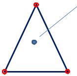
Simplex coordinates
Two-dimensional simplex coordinates:
‘1’ (x0 , y0 )
‘2’ ‘3’
Another definition of the point position is a set of simplex coordinates
1 (x0 , y0 ), 2 (x0 , y0 ), 3 (x0 , y0 )
Really only 2 of 3 simplex coordinates are independent:
General relation for the |
1 (x0 , y0 ) 2 (x0 , y0 ) 3 (x0 , y0 ) 1 |
simplex coordinates: |
|
18

Approximation of functions inside triangles
‘1’ |
Approximated function is the potential |
U (x, y) |
|
‘2’ |
‘3’ |
Electric field intensity |
|
E(x, y) U (x, y) |
|
||
|
|
|
|
||||
|
|
Ex (x, y) |
U (x, y) |
Ey (x, y) |
U (x, y) |
|
|
|
|
x |
|
|
y |
|
|
|
Potential inside a triangle: |
~ |
3 |
|
|
||
|
|
|
|
||||
|
|
(x, y) Ui i (x, y) |
|
||||
|
~ |
|
|
U |
|
||
Wave sign U means ‘approximation’ |
|
||||||
|
|
|
|
|
i 1 |
|
|
|
|
Finite function: i (x, y) ai bi x ci y |
|
|
|||
Approximation of |
~ |
3 |
|
~ |
3 |
|
|
Ex (x, y) Ui bi |
Ey (x, y) Ui ci |
|
|||||
the field intensity: |
|
i 1 |
|
i 1 |
19 |
||

Approximation of the equation
Potential inside a triangle: |
|
~ |
(x, y) |
3 |
U |
|
|
(x, y) |
||
|
U |
|
i |
|||||||
~ |
|
|
|
|
|
|
i |
|
||
Wave sign U means ‘approximation’ |
|
|
|
i 1 |
|
|
|
|
||
Finite function: |
i (x, y) ai bi x ci y |
|
|
|
|
|||||
|
2U (x, y) |
2U (x, y) |
|
|
|
|
|
|
‘1’ |
|
Equation: |
0 |
|
|
|
|
|
|
|
||
|
x2 |
y2 |
|
|
|
|
|
|
|
|
If we substitute approximation of the |
|
|
‘2’ |
|
|
‘3’ |
||||
potential into this equation we will |
|
|
|
|
|
|
|
|
||
loose information completely, because: |
|
|
|
|
|
|
||||
2 (x, y) |
2 (x, y) 0 |
|
- always! |
What to do? |
||||||
x2 |
y2 |
|
|
|
|
|
|
|
|
20 |