Учебное пособие 1944

Therefore the displacement W at S using a linear load distributed along the triangle is

WS ( ) 1 Ev2 (J1 J2 J3 ) .

Finally the element b(i, j) of the flexibility matrix of the foundation equals the displacement in the node Mi of the basic load ej(x, y). Hence

b(i, j) WMi k ,

where all the division triangles of a contact area with the node Mj as their top are summed. 4. Results of a numerical experiment. Based on the formulas a calculation software was developed for elastic foundation slab which will be dealt with in a separate paper. Here we show the application of the formulas using the example of calculating a reaction of an elastic foundation as a rigid absolutely smooth punch is pressed into it vertically. For the solution we use the above discrete equivalent

(3) the equations (2) where h = h(x, y) is piecewise-linear approximation of the density of a foundation reaction to be determined and w is the deformation (heaving) of the foundation. Small deformations are definitely investigated that in this example coincides with the heaving of the same rigid punch and are thus equal a constant under the punch and zero outside it. In order to identify h we only need to solve a linear system (3) with the known right part w.

61

Scientific Herald of t he Voronezh State University o f Architecture and Civil Engineering. Construction and Architecture

symmet rical to all ow for solutions enabling a more simple Holetsky method compar ed to the Hausse method.

Fig. 2, 3 shows t at in mos of an elastic semi-space under the punch , the stress of the foundation, reaction of a foun dation is sm all and alm ost constant. As we move from th e city to the boundary, the foundation reaction starts dropping slowly and insignificantly, then d ecreases quite abruptly and hen is slowly on the rise dramatically. Along the entire boundary of a square

a semipace detaching from t he punch as w grounds outside its boundary is not quite correct.

62

2.Aleynikov S. M., Nekrasova N. N. Contact Problem for Orthotropic Foundation Slabs with Consideration of Deformation Peculiarities of Spatial and Nongomogeneous Bases. Studia Geotechnica et Mechanica, 1998, vol. XX, no. 1—2, pp. 63—104.

3.Kachamkin A. A., Tsukrov I. I., Shvayko N. Yu. [Application of the finite element method to the calculation of anisotropic plates with variable rigidity on elastic basis]. Trudy «Voprosy prochnosti i plastichnosti» [Proc. "Problems of strength and plasticity"]. Dnepropetrovsk, 1987, pp. 30—39.

4.Aleynikov S. M., Sedaev A. A. Dual'nye setki i ikh primenenie v metode granichnykh elementov dlya resheniya kontaktnykh zadach teorii uprugosti [Dual meshes and their application in the boundary element method for the solution of contact problems of elasticity theory]. Zhurnal vychislit. matematiki i mat. fiziki, 1999, no. № 39 (2), pp. 239—253.

5.Aleynikov S. M., Sedaev A. A. Algoritm generatsii setki v metode granichnykh elementov dlya ploskikh oblastey [The algorithm of mesh generation in the boundary element method for flat areas]. Matematicheskoe modelirovanie, 1995, vol. 7, no. 7, p. 81.

6.Aleynikov S. M., Sedaev A. A. Implementation of Dual Grid Technique in BEM Analysis of 2D Contact Problems. Computer Assisted Mechanics and Engineering Sciences, 2000, vol. 7, no. 2, pp. 167—184.

63

Scientific Herald of the Voronezh State University of Architecture and Civil Engineering. Construction and Architecture

ARCHITECTURE OF BUILDINGS AND STRUCTURES.

CREATIVE CONCEPTIONS OF ARCHITECTURAL ACTIVITY

UDC 72.01

S. A. Stessel'

IMPLEMENTATION OF COMPUTER MODELING METHODS IN THE DESIGN OF NONLINEAR ARCHITECTURE OBJECTS

Scientific Research and Construction Institute for Civil Construction LTD «LENNIIPROYEKT» Russia, Saint-Petersburg, tel.: +7-921-55-77-947, e-mail: siarheistsesel@gmail.com

Leading Architect M-3

Statement of the problem. A systematization of modern computer-based methods of envelope surface geometrical modeling (system of bearing structures and enclosure which form exterior face surfaces) which are used in nonlinear architecture is necessary. Consideration of problems of geometrical surfaces which can be used as a base of spatial structures and coverings.

Results. A comprehensive analysis of possible variants of complex form computer modeling in nonlinear architecture has been developed. The methods have been described which allow a designer to create on the basis of specified geometrical model parameters. The work also features a study of their physical characteristics by means of numerical procedure and visual effects generation of complex computation. Possible ways of effective implementation of computer modeling capabilities have been outlined. The method can be used to tackle a wide range of design projects.

Conclusion. The main types of envelope forming in architecture of buildings and structures have been determined, the method of optimization of complex forms surface modeling process in architectural design has been proposed.

Keywords: nonlinear architecture, geometric modeling, methods of surface modeling.

Introduction

Architects these days are making use of new software model of designing shape as there are more and more powerful technologies offering countless opportunities. Obviously in modern architecture complex shapes are becoming more aesthetically appealing with calculation software dealing with them increasingly easier.

© Stessel' S. А., 2015

64

According to Professor of the History of Architecture and Technology at the GSD Antoine Picon, computing technology should now be viewed as a cultural phenomenon that has fundamentally changed a modern lifestyle around the world. It is now not about whether it is good or bad to use computing technology in engineering practices but about which way architecture will take influenced by it [1].

It is becoming increasingly important to design spatial computer models to detect and understand shape generated by abstract ideas in painting, biology and mathematics or nonlinear sciences. Modern architectural objects are so important that they could not be designed employing traditional methods. A lot of research has to be done prior to designing them, mathematical algorithms and logical conditions meeting specific requirements have to be created. There are still constructional, aesthetical, functional aspects to this. However, a shape does not just have to be designed but also modelled and strategically described.

It is first of all in human’s mind where modelling takes place, a general conception is used for mental images and then they take shape using a computer model. It should be noted that an advantage of a computing approach is that the technology of modelling itself is capable of transforming the original image.

There are a lot of factors influencing search of an optimal solution of the shape of a envelope. It is mostly based on functional and technological as well as compositional and planning tasks at hand. Aesthetics is of importance as well, which involves searching for an expression, perfect general proportions, rhythmic divisions (glazing and cladding “grid”) of the envelope surface. A good choice of the envelope shape assists the solution of construction tasks. It was a Spanish engineer A.Torroja argued that the best structure is the one that is reliable due to its shape but not the strength of its material [2].

Computer modelling and graphics are underpinned by two fundamental subjects, i.e. analytical geometry and optics brought together by the art of programming [3]. The tools are software complexes CAD, CAM, CAE, etc. A common element of all of these systems is a mathematical model of the geometry of an object being designed. A theoretical foundation of geometric modelling is differential and analytical geometry, variational calculation, topology and areas of computational mathematics [4]. A shape in computational mathematics is designed based on geometric parameters of structures and envelopes specified according to surfaces. A theoretical researcher of architecture J. Kipnis wrote: “No cultural practice owes so much to a technological apparatus of another practice as architecture does to geometry” [5].

65

Scientific Herald of the Voronezh State University of Architecture and Civil Engineering. Construction and Architecture

1. Classification of surfaces. In order to get a full insight into a variety and properties of surfaces that can be designed by means of geometric modelling, their classification has to be studied. There is currently a number of types of classifications of surfaces. In descriptive geometry surfaces are commonly divided into two major types – smooth and folded. In differential geometry depending on the Gaussian curvature there are surfaces with negative curvature (hyperboloids), with zero curvature (cylinders) and with positive curvature (spheres).

Depending on the method of designing a shape, there can be the following groups of surfaces: transfer, rotation, linear, non-linear and combined ones. Groups of linear surfaces can be developable (cone-shaped, torse, cylindrical) and skewed (with two or three guides) and nonlinear ones can be quadratic, cyclic, high-order surfaces and transcendental [6]. A detailed classification of surfaces (Fig. 1) set forth by S.N. Krivoshapko and V.N. Ivanov includes 38 types consisting of subtypes (they are not included in the Figure) [7].

Fig. 1. Classification of surfaces set forth by S.N. Krivoshapko and V. N. Ivanov

66

Fig. 2 shows what the classification of s urfaces depending on method o f designing in CAD and co puter graphics [4].

Depending on a te chnology of designing a model there are two types of so ftware mo delling – surface and solid. In both cases an envelope (or a few) is/are u sed to des ribe a surface. The

There are different technologies of software modelling that hel to specify an envelope (Table

Fig. 2. Classification of s urfaces in CA D and comp uter graphics

67

Scientific Herald of the Voronezh State University of Architecture and Civil Engineering. Construction and Architecture

In order to design an accurate and detailed project of envelopes Rhinoceros + + Grasshopper (Robert McNeel & Associates), Revit + Dynamo (Autodesk) can be employed. By exporting the data into other applications construction calculations can be performed and models for production as well as photo-realistic visualization can be designed.

Generally in designing complex geometric objects obtained as a result of transformations of more simple ones are employed. “Transformation” is what is done with an object or their groups to create a new geometric object. What changes an object without changing its nature is called modification or editing (replacement, rotation, scaling, mirror reflection, change of a shape). Therefore editing of an object is changing its data for a constant structure. Geometric objects are described by scalar values and vectors and editing is changing scalars and vector components.

Modelling an object can include designing one of some bodies (selection) sometimes using different operations – Boolean, rounding, joining, flatting. Different modificators (bending, rotation, etc.) can be applied. It should be noted that crossing curved lines and surfaces are

68

fundamental as there are involved in most operations on geometric objects in parametric modelling.

3. Free surfaces. Computer technologies allowing one to design complex shapes were borrowed from autoand aviadesign. In designing Guggenheim Museum in Bilbao the software CATIA was used which is common in ship and machine building, spacecraft and military industries. Using CATIA, Gehry Technologies (co-finder and head F.Gehry) designed BIM-software package Digital Project for modelling so-called free surfaces. Digital Project is widely used in designing non-linear objects. In particular, it was employed in designing the Beijing National Stadium (“Bird’s Nest”), Soumaya Museum in Mexico City, National Museum of Qatar.

Free surfaces are those different from canonic ones (a cube, plane) that can be obtained by dragging a profile along a three-dimensional curved line, designing a spline surface using control points, smooth joining of two pieces, etc. Hence technologies for designing free surfaces originally used for mechanical engineering (designing complex technical objects, e.g., blades of a turbine, an aircraft fuselage are currently employed in architectural designing while modelling envelope surfaces.

Depending on certain characteristics there are three classes of surfaces — A, B, C [8] (Table 2).

69

Scientific Herald of the Voronezh State University of Architecture and Civil Engineering. Construction and Architecture

Class А surfaces (aesthetic surfaces) is a term used in designing and engineering to denote a set of free surfaces with special requirements to accuracy and quality of modelling. Particularly they are made using highly smooth pieces at joining points where not only tangents of surfaces but curvatures need to coincide (G2, G3 curvature continuity where 2 and 3 denote smoothness) (Table 3).

Free surfaces are designed based on modelling using curved lines by means of different operations (lofting, profile squeezing, etc.) or by editing a surface, e.g. using control points.

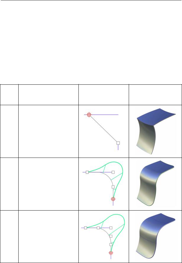
Table 3

Types of surface continuity

Type

of surface Description Scheme Image continuity

Position of a point is determined

G0

not only by its position at the joining. Two curved lines come in contact at final points

Tangent determines the position and direction of a curved line at

G1

final points. Two curved lines not only come in contact but they also move in the same direction in relation to a tangent point

Continuity of curvature between two curved lines determines the position, direction and radius of G2 curvature at final points. Curved lines at the joint do not just move in the same direction but they also have the same radius at final points

70